Atlases
A brain atlas ties every voxel of a reference volume to a named region. In ConfUSIus an
atlas is a plain xarray.Dataset with three data variables on a
common (z, y, x) grid (reference, the
template volume; annotation, integer
region labels; and hemispheres, 1 = left,
2 = right), plus an .atlas accessor that
carries all atlas-aware operations. The structure hierarchy rides along in
Dataset.attrs["structures"], so a single object fully describes the atlas and its
region tree.
BrainGlobe Atlases
ConfUSIus does not ship its own atlases. It builds on the
BrainGlobe Atlas API,
which packages dozens of community atlases behind one interface, and
fetch_brainglobe_atlas fetches any of them
by name:
The first call downloads the atlas through BrainGlobe and caches it in BrainGlobe's own
cache (~/.brainglobe, shared with other BrainGlobe tools); later calls read from the
cache. Any name from the
BrainGlobe atlas list
works, covering mouse, rat, human, zebrafish, and more, at several resolutions.
The returned object is the Dataset described above:
>>> atlas
<xarray.Dataset> Size: 11MB
Dimensions:      (z: 132, y: 80, x: 114)
Coordinates:
  * z            (z) float64 1kB 0.0 0.1 0.2 0.3 0.4 ... 12.8 12.9 13.0 13.1
  * y            (y) float64 640B 0.0 0.1 0.2 0.3 0.4 ... 7.5 7.6 7.7 7.8 7.9
  * x            (x) float64 912B 0.0 0.1 0.2 0.3 0.4 ... 11.0 11.1 11.2 11.3
Data variables:
    reference    (z, y, x) float32 5MB 0.0 0.0 0.0 0.0 0.0 ... 1.0 1.0 1.0 1.0
    annotation   (z, y, x) int32 5MB 0 0 0 0 0 0 0 0 0 0 ... 0 0 0 0 0 0 0 0 0 0
    hemispheres  (z, y, x) int8 1MB 2 2 2 2 2 2 2 2 2 2 ... 1 1 1 1 1 1 1 1 1 1
Attributes:
    name:              allen_mouse
    citation:          Wang et al 2020, https://doi.org/10.1016/j.cell.2020.0...
    species:           Mus musculus
    orientation:       asr
    structures:        root (997) ...
    physical_to_base:  [[1. 0. 0. 0.] ...
Coordinates are in millimeters, so an atlas plots and registers against fUSI recordings directly.
Building your own atlas
Because ConfUSIus leans on the BrainGlobe atlas format, a custom atlas (for example
a coarse parcellation for functional connectivity) is best authored as a BrainGlobe
atlas and then loaded with the same fetch_brainglobe_atlas call. BrainGlobe's
Adding a new atlas
guide and the atlas_scripts in the
brainglobe-atlasapi repository
walk through packaging a reference stack, an annotation stack, and a structure
hierarchy into a distributable atlas.
Exploring the Structure Hierarchy
Regions form a tree: root contains gray and white matter, which contain areas, which
contain layers. show_tree prints the whole
hierarchy, and its nid argument restricts the printout to one branch, which is handy
since the full Allen tree has well over a thousand nodes:
HIP (1080)
├── CA (375)
│   ├── CA1 (382)
│   ├── CA2 (423)
│   └── CA3 (463)
├── DG (726)
│   ├── DG-mo (10703)
│   ├── DG-po (10704)
│   └── DG-sg (632)
├── FC (982)
└── IG (19)
Indexing structures by acronym (or integer id) returns the BrainGlobe record for a
region, including its full path from the root:
>>> atlas.structures["HIP"]
{'acronym': 'HIP',
 'id': 1080,
 'name': 'Hippocampal region',
 'structure_id_path': [997, 8, 567, 688, 695, 1089, 1080],
 'rgb_triplet': [126, 208, 75],
 'mesh_filename': PosixPath('.../allen_mouse_100um_v1.2/meshes/1080.obj')}
ancestors returns the same path as tree
nodes, from the root down to (but excluding) the region:
>>> [node.tag for node in atlas.atlas.ancestors("HIP")]
['root (997)', 'grey (8)', 'CH (567)', 'CTX (688)', 'CTXpl (695)', 'HPF (1089)']
Looking Up and Searching Regions
lookup flattens the hierarchy into a
pandas.DataFrame indexed by region id, with the acronym, full name,
and RGB color of every structure:
>>> atlas.atlas.lookup.head()
       acronym                           name      rgb_triplet
id
997       root                           root  [255, 255, 255]
8         grey  Basic cell groups and regions  [191, 218, 227]
567         CH                       Cerebrum  [176, 240, 255]
688        CTX                Cerebral cortex  [176, 255, 184]
695      CTXpl                 Cortical plate  [112, 255, 112]
Region acronyms are terse, so search finds
structures by substring or regex. By default it matches both the acronym and the name
(case-insensitive):
>>> atlas.atlas.search("visual").head()
       acronym                                  name    rgb_triplet
id
669        VIS                          Visual areas  [8, 133, 140]
402      VISal             Anterolateral visual area  [8, 133, 140]
1074    VISal1    Anterolateral visual area, layer 1  [8, 133, 140]
905   VISal2/3  Anterolateral visual area, layer 2/3  [8, 133, 140]
1114    VISal4    Anterolateral visual area, layer 4  [8, 133, 140]
Pass field="acronym" (or "name") to match one column exactly with a regex, useful for
pinning down a single area without its layer subdivisions:
>>> atlas.atlas.search("VISp", field="acronym")
    acronym                 name    rgb_triplet
id
385    VISp  Primary visual area  [8, 133, 140]
search,
get_masks, and
get_mesh are also exposed as free functions
in confusius.atlas that take the Dataset as their first argument, so
cf.atlas.search_atlas(atlas, "visual") is equivalent to atlas.atlas.search("visual"). Both
forms validate the Dataset as an atlas before running.
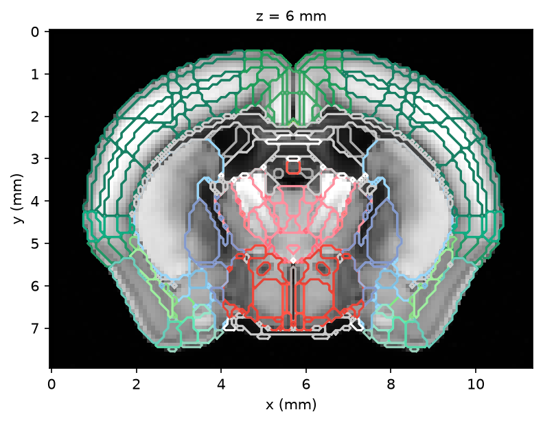
Plotting Annotations over the Reference
The reference and annotation volumes plot with the ordinary
plot_volume tools. Overlaying the region boundaries on
a reference slice with add_contours
gives the familiar atlas view; contour colors come from each region's atlas color
automatically:
plotter = cf.plotting.plot_volume(
    atlas.atlas.reference.sel(z=slice(6, 6)), show_colorbar=False
)
plotter.add_contours(atlas.atlas.annotation.sel(z=slice(6, 6)))
Region Surface Meshes
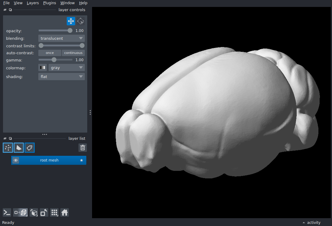
Many BrainGlobe atlases bundle a triangular surface mesh per region.
get_mesh returns the mesh as a (vertices,
faces) pair in the atlas's physical space (millimeters), ready to hand to any 3D viewer.
napari's add_surface takes exactly that pair:
import napari

surface_data = atlas.atlas.get_mesh("root")
napari.Viewer(ndisplay=3).add_surface(surface_data)
Pass side="left" or side="right" to clip the mesh to one hemisphere. Because meshes
come back in the atlas's current physical space, they stay aligned with the volumes after
a resample (see below).
Masks for Regional Analysis
get_masks turns regions into integer voxel
masks stacked along a mask dimension, automatically including every descendant in the
hierarchy. Pass one region or many, and optionally restrict each to a hemisphere:
>>> atlas.atlas.get_masks(["VISp", "AUDp", "MOp"])
<xarray.DataArray (mask: 3, z: 132, y: 80, x: 114)> Size: 14MB
0 0 0 0 0 0 0 0 0 0 0 0 0 0 0 0 0 0 0 ... 0 0 0 0 0 0 0 0 0 0 0 0 0 0 0 0 0 0 0
Coordinates:
  * mask     (mask) <U4 48B 'VISp' 'AUDp' 'MOp'
  * z        (z) float64 1kB 0.0 0.1 0.2 0.3 0.4 ... 12.7 12.8 12.9 13.0 13.1
  * y        (y) float64 640B 0.0 0.1 0.2 0.3 0.4 0.5 ... 7.5 7.6 7.7 7.8 7.9
  * x        (x) float64 912B 0.0 0.1 0.2 0.3 0.4 ... 10.9 11.0 11.1 11.2 11.3
Attributes:
    rgb_lookup:  {997: [255, 255, 255], 8: [191, 218, 227], 567: [176, 240, 2...
    roi_labels:  {997: 'root (root)', 8: 'Basic cell groups and regions (grey...
    cmap:        <matplotlib.colors.ListedColormap object at 0x71ba5c798050>
    norm:        <matplotlib.colors.BoundaryNorm object at 0x71ba5cb3f230>

>>> left_hip = atlas.atlas.get_masks("HIP", sides="left")
>>> left_hip.mask
<xarray.DataArray 'mask' (mask: 1)> Size: 20B
'HIP_L'
Coordinates:
  * mask     (mask) <U5 20B 'HIP_L'
These masks feed directly into signal extraction and connectivity; see the examples Atlas-based region correlation matrix and Atlas-based seed connectivity maps for more.
Aligning an Atlas to a Recording
An atlas is only useful once it shares a grid with your data. After registering a
recording to the atlas template (see Registration),
resample_like warps the reference,
annotation, hemisphere map, and region meshes onto the recording's grid in one call,
using an affine, B-spline, or displacement-field transform from
register_volume:
Resampling can be costly, so it is worth doing once and caching the result.
save_atlas / load_atlas write
the whole atlas (arrays, structure hierarchy, and region meshes) to a Zarr store and
read it back ready to use. The
Register a recording to an Allen fUSI template
example walks through the full register → resample → save → reload workflow.
API Reference
For full parameter documentation, see the atlas API reference and the
I/O API reference for save_atlas/load_atlas.