Using the Plugin
The ConfUSIus sidebar contains six collapsible panels. Each panel operates independently and can be expanded or collapsed by clicking its header. For an in-app introduction, click Take a Tour in the sidebar header.
- Data I/O — load and save fUSI files (NIfTI, Zarr, SCAN).
- Video — load videos side-by-side, temporally synced with the fUSI acquisition.
- Signals — plot voxel, point, or label-region signals in a bottom dock.
- Events — annotate periods of time (BIDS events) and shade them on the signal plot.
- QC — compute DVARS, carpet, CV, tSNR for a selected layer.
- Registration — run between-scan or within-scan registration, inspect progress, and save/apply transforms.
Data I/O Panel
The Data I/O Panel handles both loading and saving fUSI files without leaving the viewer.
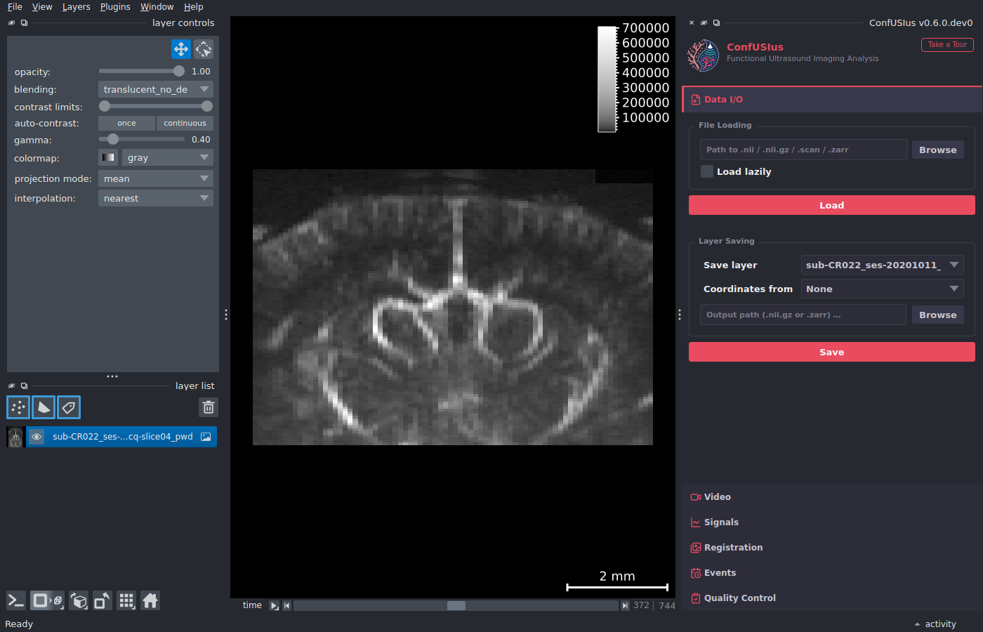
Loading data
Click Browse to pick a file—it loads immediately on selection. Or paste a path directly in the text field and press Enter. Enable Load lazily beforehand to keep the array Dask-backed for large files. A progress bar animates during loading, and any error is reported in the napari notification bar.
Time overlay
When a loaded scan contains a time dimension, the current time coordinate is displayed as a text overlay in the bottom-left corner of the canvas. The value and units are read from the scan's coordinate metadata and update automatically as you scrub the time slider.
When multiple scans are open, the overlay reflects the currently selected layer. If zero or more than one layer is selected, it keeps following the previously selected one.
Saving data
- Select the layer to save from the Save layer dropdown.
- Optionally select a layer in the Coordinates from dropdown to borrow its physical coordinates and attributes. This is useful when saving a labels layer drawn on top of a fUSI image: selecting the image layer as the template preserves the full physical coordinate system. If the labels layer has fewer dimensions than the template (e.g. a 3D labels layer against a 4D image), the trailing spatial dimensions are used automatically.
- Type an output path or click Browse. The format is inferred from the extension:
.nii/.nii.gzfor NIfTI and.zarrfor Zarr. - Click Save. A notification confirms success.
Three save modes are applied automatically depending on what is available:
| Mode | When applied |
|---|---|
| Direct | The layer was loaded via ConfUSIus (DataArray in metadata). Saved verbatim, all coordinates and attributes preserved. |
| Template | A template layer is selected. Coordinates are borrowed from the template DataArray. |
| Reconstruct | No template and no DataArray in metadata (e.g. a freshly drawn labels layer). Coordinates are reconstructed from the napari layer state (scale, translate, axis_labels). |
Video Panel
The Video Panel loads one or more videos (.mp4, .mov, .avi) and
overlays them beside a fUSI scan in a synchronized grid. Each video becomes its own
napari Image layer whose time axis is locked to the reference scan, so scrubbing the
time slider plays every video in lockstep with the fUSI recording.
Loading a video
- Pick the fUSI image layer to synchronize against in the Reference layer
dropdown. The reference must have ConfUSIus coordinate metadata, so load it
through the Data I/O Panel or the
confusiusCLI command. - Insert a path or click Browse to pick a video file.
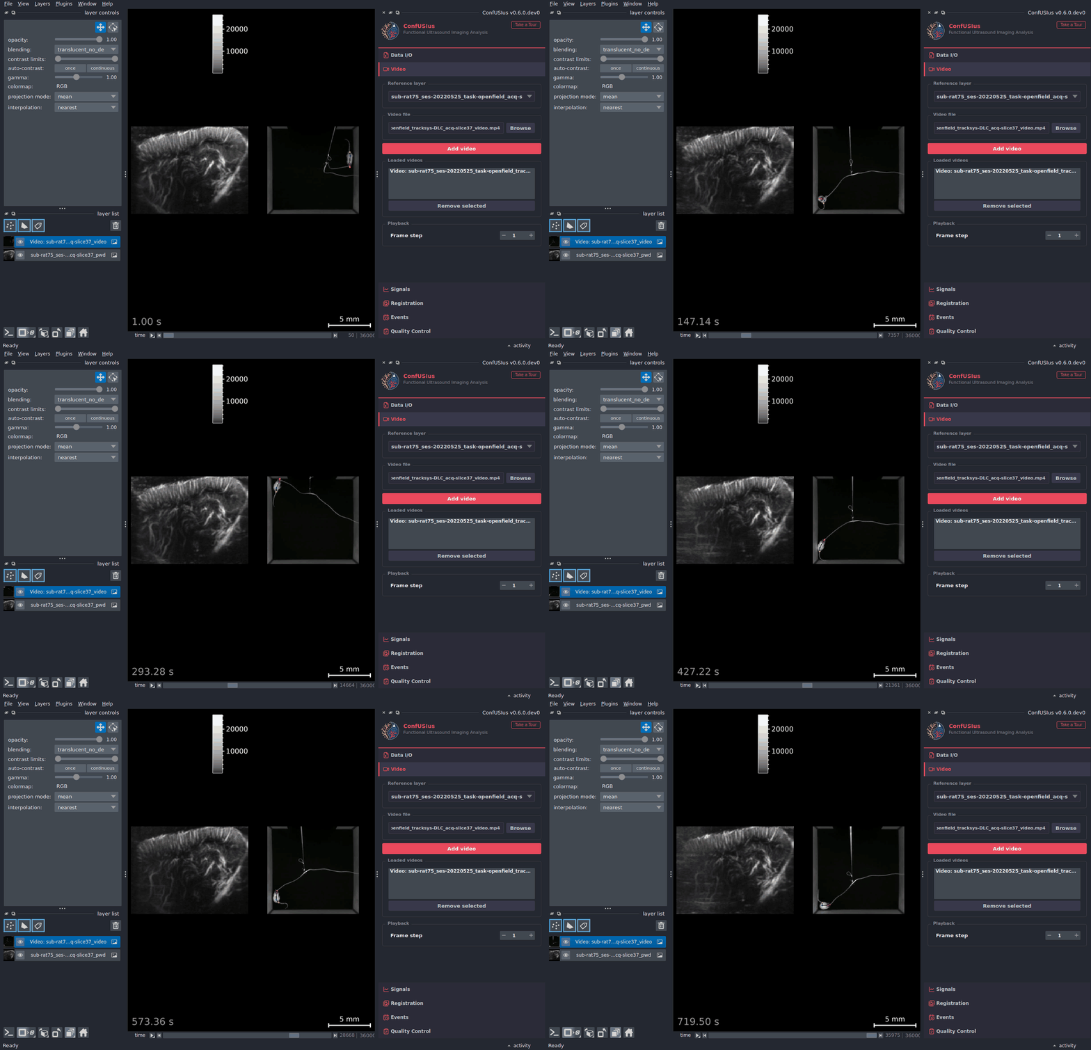
- Click Add video. The video appears as a new Image layer, grid mode is enabled with a single-row layout, and the viewer shows the reference scan and the video side by side.
Repeat to add more videos (each will get its own cell). All videos share the reference layer's axis labels, time index, and dimensionality; their spatial scale is chosen so the video height matches the fUSI height, with isotropic pixels and the frame centered on the scan.
Launch with a video from the CLI
Pass both a data file and --video to open them together:
Playback
| Option | Description |
|---|---|
| Frame step | Show every N-th frame of the video. Higher values skip frames for lighter playback of long or high-frame-rate recordings. The effective frame rate becomes fps / N. Changes apply to every loaded video. |
Napari playback performance
Napari handles animations quite smoothly up to around 30 to 50 FPS (even higher depending on user hardware and operating system). Use Frame step to reduce the effective frame rate if playback is choppy or buffering.
The time scale of each video layer is frame_step / fps seconds, so the napari
time slider and the time overlay continue to report physical seconds regardless
of the chosen step.
Time axis is kept out of the displayed dims
The panel installs a guard that prevents napari from ever placing the time axis in the 2D display. If you reorder dimensions such that time would become a display dimension, the order is silently corrected.
Signals Panel
The Signals Panel plots signals extracted from image layers along any non-spatial dimension (time, lag, feature, etc.). The plot appears in a bottom dock that is created the first time you click Show Signal Plot.
Choosing a data source
Pick one of three source modes in the Source group:
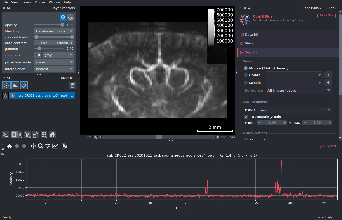
- Mouse
- Hold Shift and move the mouse over the canvas. The plot updates live with the single-voxel signal at the cursor position.
- Points
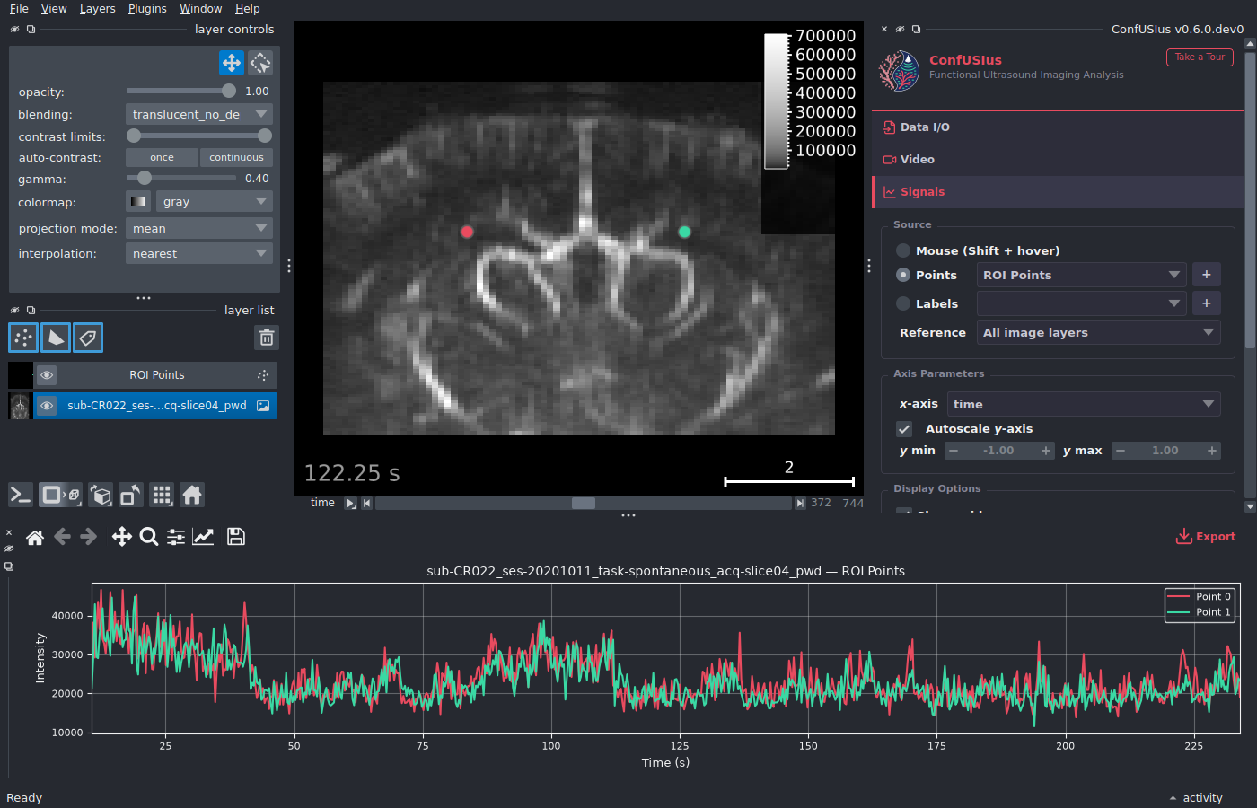
- Select a Points layer from the dropdown (or click + to create one). Each point is plotted as a separate line colored by its face color. Add or remove points in napari and the plot updates automatically.
- Labels
- Select a Labels layer from the dropdown (or click + to create one). The mean signal is extracted for each distinct non-zero label and plotted as a separate line, colored by the label's color in the napari colormap. This is useful for quickly comparing region-averaged signals after painting ROIs with napari's brush tool.
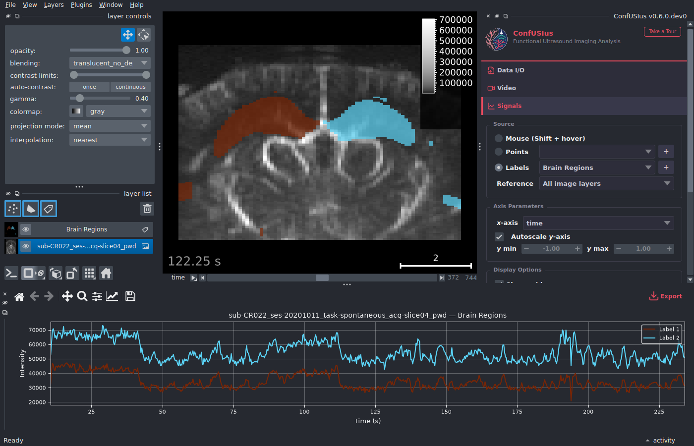
In Points and Labels modes, the Reference dropdown selects which image layer to extract signals from. It defaults to All image layers, which plots each layer as a separate line (distinguished by line style).
Axis parameters
| Option | Description |
|---|---|
| x-axis | Choose which non-spatial dimension to plot on the horizontal axis. Defaults to time when available, otherwise the first non-spatial dimension. |
| y min / y max | Manual limits for the vertical axis (disabled while autoscale is on). |
| Autoscale y-axis | When enabled, the vertical axis rescales to fit the data automatically. Disabling it captures the current limits so you can fine-tune them. |
Display options
| Option | Description |
|---|---|
| Show grid | Show or hide the background grid. |
| Show x-axis cursor | Draw a vertical line on the plot that follows the napari dimension slider for the selected x-axis dimension. |
| Z-score signal | Normalize each signal to zero mean and unit variance before plotting. The y-axis label changes from "Intensity" to "Z-score". |
Click to navigate
Left-click anywhere on the signal plot to jump the napari viewer to the corresponding time slice. Clicks are ignored while a zoom or pan tool is active in the plot toolbar.
Managing signals
Click Manage Signals to open a floating dialog where you can customize both live signals (from the current source mode) and imported signals:
- Rename: Double-click a signal's name to edit it.
- Recolor: Click the color swatch to pick a new color. Changes are synced back to the napari layer (point face color or label colormap).
- Show / Hide: Toggle individual signal visibility with the checkbox.
Importing and exporting signals
- Import
- In the Manage Signals dialog, click Import to load one or more signal files at
once. Standard CSV / TSV files must contain a column whose header matches the
current x-axis dimension name (e.g.
time) plus one or more numeric value columns. BIDS physio files ending in_physio.tsv.gzare also supported: ConfUSIus reads their JSON sidecar, uses the declared column names, and synthesizestimefromSamplingFrequencyandStartTimewhen needed. Each value column becomes a separate signal overlaid on the plot. - Export
- Click the Export button in the plot toolbar to export all currently plotted signals—both live and imported—to a CSV or TSV file.
Events Panel
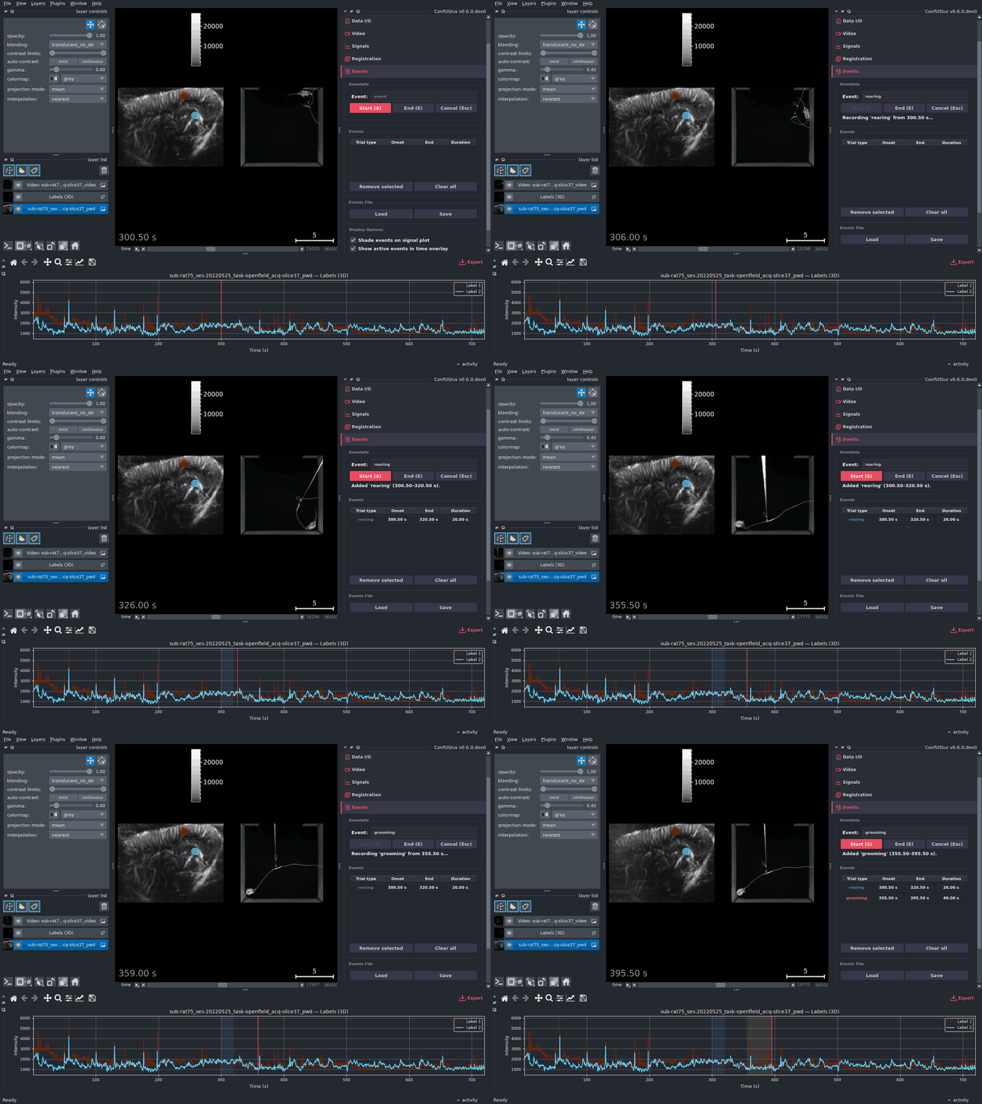
The Events Panel allows annotating periods of time—not individual frames—following the
BIDS
events
convention (onset, duration, and an optional trial_type). Annotated events shade
the signal plot and are named in the time overlay while they are
active.
Annotating events
- Type a name for the event in the Event field (defaults to
event). - Press Start (S) to mark the onset at the current time step, scrub the time slider forward, then press End (E) to mark the offset. Cancel (Esc) discards an in-progress annotation. The shortcuts are active whenever the panel is open.
- The event appears in the table with its trial type, onset, end, and duration.
The End time must not be before the Start time. Ending at the Start time creates an instantaneous (zero-duration) event, as allowed by BIDS; it is drawn as a vertical line instead of a shaded band.
Loading and saving
Use Load to import a BIDS events .tsv file (onset and duration are required; a
missing trial_type defaults to event) and Save to write the current events back
out as a BIDS events .tsv.
Straight into analysis
An events .tsv saved here is a standard BIDS events table, so it can be read back
with load_events and fed directly to either
make_first_level_design_matrix or
the fit method of a FirstLevelModel:
Display options
| Option | Description |
|---|---|
| Shade events on signal plot | Draw each event as a colored band spanning its interval on the bottom-dock signal plot, colored by trial type. |
| Show active events in time overlay | Append each active event to the time overlay as name [onset, end). An event is active while the current frame's acquisition window overlaps it. The window comes from the layer's volume_acquisition_reference/volume_acquisition_duration metadata, using the frame spacing as the duration when only the reference is present, and the frame's timestamp alone when neither is; an event too short to be sampled by any frame is shown on the next frame instead. |
QC Panel
The QC Panel computes quality control metrics for a selected image layer.
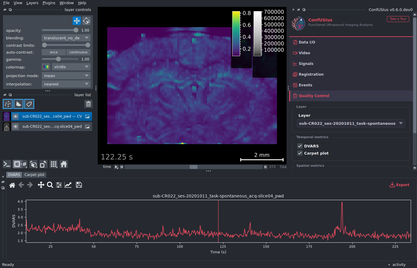
Select a layer from the Layer dropdown, check the metrics you want, and click Compute.
Temporal metrics are rendered as plots in the bottom dock (the same dock used by the Signals Panel, in separate tabs). Computed plots are cached and survive dock closure: closing and reopening the bottom dock restores the last computed result.
- DVARS
- Plots the standardized temporal derivative of variance over time. A vertical cursor follows the napari time slider. See DVARS for interpretation.
- Carpet plot
- Displays the full voxel time series as a 2D raster (time × voxels). See Carpet Plot for interpretation.
Click to navigate
Left-click anywhere on a temporal metric plot (DVARS or carpet) to jump the napari viewer to the corresponding time slice. Clicks are ignored while a zoom or pan tool is active in the plot toolbar.
Spatial map metrics are added as new image layers in the napari layer list, with correct physical scale and origin preserved.
- CV
- Coefficient of variation map.
- tSNR
- Temporal signal-to-noise ratio map.
Prefer CV over tSNR for fUSI power Doppler data
tSNR is misleading for power Doppler: low-signal regions such as gel layers and shadow zones behind the skull can appear bright. CV correctly highlights regions with high temporal variability. See the Quality Control guide for a full explanation.
Registration Panel
The Registration Panel runs the ConfUSIus registration workflows directly from napari. Use Between scans for registering different recordings, or Within-scan for volume-wise motion correction within a single recording. The panel supports modifying registration parameters, live preview, and saving/loading/applying computed transforms.
Between scans
Use Between scans when you want to register one layer onto another, for example two recordings from different animals or a functional recording onto an angiography.
- Select the Moving layer and Fixed layer.
- Choose a transform model.
- Optionally choose a Scale for to compress the intensity dynamics.
- Optionally choose an Initialization transform if layers are very misaligned.
- Click Run registration.
Available transform models are:
translationfor x/y/z-only shifts,rigidfor translations and rotations,affinefor translations, rotations, scaling, and shear,bsplinefor non-linear local deformations.
For bspline, a staged workflow usually works best: first run rigid or affine, then
run bspline and select the previous transform in Initialization. This lets the
B-spline model refine a good global alignment instead of trying to solve both
large-scale and local deformation at once.
Main parameters
| Parameter | What it does | When it is useful |
|---|---|---|
| Transform | Chooses the motion model being optimized. | Start with translation or rigid for simple alignment; use affine for global scale/shear differences; use bspline only after a good global initialization. |
| Mesh size | Sets the B-spline control-grid density. | Increase it only when bspline needs to capture finer local mismatches; too fine a grid can lead to unrealistic warping. |
| Metric | Chooses the similarity criterion (correlation or mattes_mi). |
correlation is a good default for power Doppler data; mattes_mi is more robust when intensity distributions differ. |
| Scale | Applies optional intensity scaling before registration. | Useful for power Doppler data where large vessels are typically overbright compared to finer structures. |
| Initialization | Sets the starting transform before optimization. | Use center_geometry or center_moments for coarse setup; reuse a saved/manual affine transform when you already have a good approximate alignment. |
| Learning rate | Sets the optimizer step size. | Leave Auto enabled to let SimpleITK estimate it each iteration, or untick it to use a fixed value (default 1.0). |
| Iterations | Maximum number of optimizer steps. | Increase it when alignment is still improving near the end of a run. |
Advanced parameters
| Parameter | What it does | When it is useful |
|---|---|---|
| Histogram bins | Number of bins used by mattes_mi. |
Tune only when using mutual information; more bins can capture finer intensity structure but may be noisier. |
| Convergence min | Minimum optimizer improvement required to keep iterating. | Lower it when you want stricter convergence. |
| Convergence window | Number of recent iterations used to test convergence. | Increase it to make convergence detection less sensitive to noise. |
| Multi-resolution | Runs registration from coarse to fine scales. | Usually helpful for difficult B-spline alignments or large initial offsets. |
| Shrink factors | Downsampling factors for each resolution level. | Use larger coarse levels when the initial mismatch is large. |
| Smoothing sigmas | Gaussian smoothing at each resolution level. | Helps emphasize global structure before fine alignment. |
| Resample interp. | Interpolation used for the registered output and previews. | linear is the usual default; bspline can give smoother resampled images. |
| Fill value | Value written outside the moving field of view after resampling. | Useful for controlling the appearance of padded background. |
| ITK Threads | Number of SimpleITK threads used for between-scan registration. | Reduce it when you are running several heavy jobs at once; -1 uses all CPUs. |
| Optimizer weights | Applies per-parameter optimizer weights. | Use it to freeze or down-weight specific affine parameters; not available for B-spline transforms. |
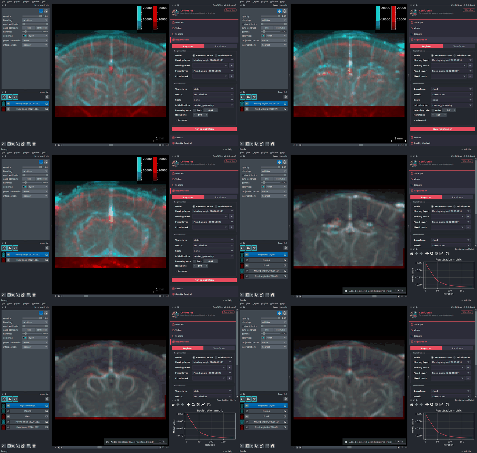
The animation below uses between-session angiography volumes from the same animal across different days. ConfUSIus keeps the original layers untouched, adds dedicated preview layers for inspection, and stores the final registered result as a new layer when the run completes.
Within-scan
Use Within-scan for motion correction inside a single time series.
- Switch Mode to Within-scan.
- Select the time-series Moving layer.
- Choose the Reference volume index used as the registration target.
- Pick a transform model (
translation,rigid, oraffine). - Click Run registration.
Main parameters
| Parameter | What it does | When it is useful |
|---|---|---|
| Reference volume | Chooses the volume index used as the motion-correction target. | Pick a representative, sharp frame with little motion. |
| Transform | Chooses the volume-wise motion model. | rigid is the safest starting point; affine is available when motion is more complex. |
| Metric | Chooses the volume-to-reference similarity criterion. | correlation is usually a good default for within-recording motion correction. |
| Scale | Applies optional preprocessing before registration. | Useful when an intensity transform makes anatomy more stable across time for the optimizer. |
| Initialization | Sets the initial volume-wise centering transform. | Most runs can use no initialization. |
| Learning rate | Sets the optimizer step size for each frame. | Within-scan uses a fixed value here; the default is 0.01. Reduce it if updates look unstable; increase it if frames are already close and convergence is too slow. |
| Iterations | Maximum optimizer steps per frame. | Increase it for harder motion or more flexible transforms. |
Advanced parameters
| Parameter | What it does | When it is useful |
|---|---|---|
| Histogram bins | Number of bins used by mattes_mi. |
Only relevant when using mutual information. |
| Convergence min | Minimum optimizer improvement required to keep iterating. | Lower it when you want stricter volume-wise convergence. |
| Convergence window | Number of recent iterations used to test convergence. | Increase it when convergence decisions look too jittery. |
| Multi-resolution | Runs each frame registration from coarse to fine scales. | Helpful when motion is large or frames are noisy. |
| Shrink factors | Downsampling factors for each resolution level. | Useful for coarse-to-fine motion correction. |
| Smoothing sigmas | Gaussian smoothing at each resolution level. | Helps stabilize coarse registration before fine refinement. |
| Resample interp. | Interpolation used for the motion-corrected output. | Controls output smoothness. |
| Fill value | Value used outside the field of view after resampling. | Mostly useful for controlling output background appearance. |
| Diagnostics | Stores full volume-wise optimizer traces. | Enable it only when you want detailed debugging or later inspection. |
| Parallel jobs | Number of workers used for volume-wise registration. | Increase it to speed up long runs; reduce it if your machine is already busy. -1 uses all available CPUs. |
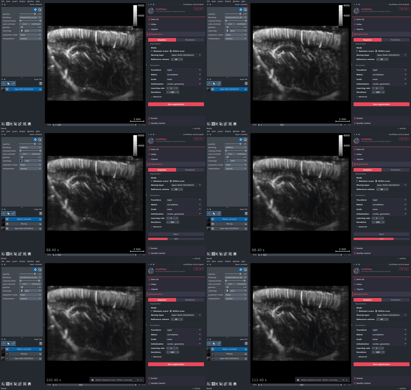
This workflow returns a Motion corrected layer and updates the progress bar as frames
finish. The animation below uses a short open-field recording chunk and shows the result
filling in progressively.