Registration of two sessions from the same subject
This example shows how to align two power Doppler images acquired from the same
subject in different sessions. We use
register_volume with a rigid transform,
which is appropriate when the imaged anatomy is the same but the probe placement
differs slightly between the two recordings.
We pick two angio acquisitions from the Cybis Pereira 2026
dataset using
fetch_cybis_pereira_2026: subject
rat75, slice slice32, recorded on consecutive days (sessions 20220523 and
20220524).
Fetch and load both recordings
Each recording is a single power Doppler image of one slice. We convert it to decibels
for both display and registration, which is usually more stable on the log-compressed
dynamic range. We also set the coordinate system to the NIfTI qform's space, because
the sform coordinate system is currently unusable as it is a custom non-metric
space.
from pathlib import Path

import matplotlib as mpl
import matplotlib.pyplot as plt
import numpy as np
import xarray as xr

import confusius as cf

# Adapt background color to the current Matplotlib style.
bg_color = mpl.colors.to_hex(mpl.rcParams["figure.facecolor"])

xr.set_options(display_expand_data=False)

sessions = ["20220523", "20220524"]
acq = "slice32"
bids_root = cf.datasets.fetch_cybis_pereira_2026(
    datasets="rawdata",
    subjects="rat75",
    sessions=sessions,
    datatypes="angio",
    acqs=acq,
)
If you use this dataset in your work, please cite the following source:

Cybis Pereira, F., Castedo, S. H., Meur-Diebolt, S. L., Ialy-Radio, N., Bhattacharya, S., Ferrier, J., Osmanski, B.
F., Cocco, S., Monasson, R., Pezet, S., & Tanter, M. (2026). A vascular code for speed in the spatial navigation
system. Cell Reports, 45(1). https://doi.org/10.1016/j.celrep.2025.116791
def _load_angio_for_registration(session: str) -> xr.DataArray:
    """Load an angio acquisition and scale its intensity for registration."""
    path = (
        Path(bids_root)
        / "sub-rat75"
        / f"ses-{session}"
        / "angio"
        / f"sub-rat75_ses-{session}_acq-{acq}_rec-minframe2d_pwd.nii.gz"
    )
    angio = cf.load(path).fusi.scale.db().compute()
    return angio.fusi.affine.apply(angio.affines["physical_to_qform"])[0]


fixed = _load_angio_for_registration(sessions[0])

fixed
- z: 1
- y: 112
- x: 128
- -19.87 -18.5 -16.81 -17.79 -14.17 ... -21.8 -21.61 -22.72 -22.63
array([[[-19.86943521, -18.49816633, -16.81460287, ..., -20.34940616, -20.95297252, -21.0594714 ], [-20.37608604, -18.82660631, -16.94106874, ..., -19.85784515, -21.06570853, -21.44495125], [-20.51718032, -20.88758297, -19.33940193, ..., -20.89870803, -22.26240509, -22.35662323], ..., [-15.87173364, -16.1433349 , -15.9975841 , ..., -20.36189552, -20.24644136, -20.41257363], [-19.52239672, -18.86263447, -18.68976199, ..., -20.05567394, -20.46102047, -20.02077658], [-21.18090479, -21.5516875 , -22.47616461, ..., -21.60698958, -22.72244543, -22.63380267]]], shape=(1, 112, 128)) - z(z)float64-7.105e-15
- units :
- mm
- voxdim :
- 0.3999999761581421
array([-7.105427e-15])
- y(y)float645.0 5.099 5.197 ... 15.84 15.94
- units :
- mm
- voxdim :
- 0.09855999797582626
array([ 5. , 5.09856, 5.19712, 5.29568, 5.39424, 5.4928 , 5.59136, 5.68992, 5.78848, 5.88704, 5.9856 , 6.08416, 6.18272, 6.28128, 6.37984, 6.4784 , 6.57696, 6.67552, 6.77408, 6.87264, 6.9712 , 7.06976, 7.16832, 7.26688, 7.36544, 7.464 , 7.56256, 7.66112, 7.75968, 7.85824, 7.9568 , 8.05536, 8.15392, 8.25248, 8.35104, 8.4496 , 8.54816, 8.64672, 8.74528, 8.84384, 8.9424 , 9.04096, 9.13952, 9.23808, 9.33664, 9.4352 , 9.53376, 9.63232, 9.73088, 9.82944, 9.928 , 10.02656, 10.12512, 10.22368, 10.32224, 10.4208 , 10.51936, 10.61792, 10.71648, 10.81504, 10.9136 , 11.01216, 11.11072, 11.20928, 11.30784, 11.4064 , 11.50496, 11.60352, 11.70208, 11.80064, 11.8992 , 11.99776, 12.09632, 12.19488, 12.29344, 12.392 , 12.49056, 12.58912, 12.68768, 12.78624, 12.8848 , 12.98336, 13.08192, 13.18048, 13.27904, 13.3776 , 13.47616, 13.57472, 13.67328, 13.77184, 13.8704 , 13.96896, 14.06752, 14.16608, 14.26464, 14.3632 , 14.46176, 14.56032, 14.65888, 14.75744, 14.856 , 14.95456, 15.05312, 15.15168, 15.25024, 15.3488 , 15.44736, 15.54592, 15.64448, 15.74304, 15.8416 , 15.94016]) - x(x)float64-6.985 -6.875 ... 6.875 6.985
- units :
- mm
- voxdim :
- 0.10999999940395354
array([-6.985, -6.875, -6.765, -6.655, -6.545, -6.435, -6.325, -6.215, -6.105,
       -5.995, -5.885, -5.775, -5.665, -5.555, -5.445, -5.335, -5.225, -5.115,
       -5.005, -4.895, -4.785, -4.675, -4.565, -4.455, -4.345, -4.235, -4.125,
       -4.015, -3.905, -3.795, -3.685, -3.575, -3.465, -3.355, -3.245, -3.135,
       -3.025, -2.915, -2.805, -2.695, -2.585, -2.475, -2.365, -2.255, -2.145,
       -2.035, -1.925, -1.815, -1.705, -1.595, -1.485, -1.375, -1.265, -1.155,
       -1.045, -0.935, -0.825, -0.715, -0.605, -0.495, -0.385, -0.275, -0.165,
       -0.055,  0.055,  0.165,  0.275,  0.385,  0.495,  0.605,  0.715,  0.825,
        0.935,  1.045,  1.155,  1.265,  1.375,  1.485,  1.595,  1.705,  1.815,
        1.925,  2.035,  2.145,  2.255,  2.365,  2.475,  2.585,  2.695,  2.805,
        2.915,  3.025,  3.135,  3.245,  3.355,  3.465,  3.575,  3.685,  3.795,
        3.905,  4.015,  4.125,  4.235,  4.345,  4.455,  4.565,  4.675,  4.785,
        4.895,  5.005,  5.115,  5.225,  5.335,  5.445,  5.555,  5.665,  5.775,
        5.885,  5.995,  6.105,  6.215,  6.325,  6.435,  6.545,  6.655,  6.765,
        6.875,  6.985])
- sform_code :
- 5
- qform_code :
- 1
- clutter_filter_window_duration :
- 200
- clutter_filters :
- ['svd:remove_first_60_components']
- IsHadamard :
- True
- manufacturer :
- Iconeus
- manufacturers_model_name :
- Iconeus One
- plane_wave_angles :
- [-3.0, -1.0, 1.0, 3.0]
- power_doppler_integration_duration :
- 200
- probe_central_frequency :
- 15.625
- ProbeElevationAperture :
- 1.5
- ProbeElevationFocus :
- 8
- probe_model :
- IcoPrime light
- probe_number_of_elements :
- 128
- probe_pitch :
- 0.11
- probe_radius_of_curvature :
- 0
- probe_type :
- linear
- probe_voltage :
- 15
- UltrafastSamplingFrequency :
- 500.0
- pulse_repetition_frequency :
- 2000.0
- affines :
- {'physical_to_sform': array([[ 1.28309483e-17, -5.62707691e-03, 1.15276755e-01, -2.23374989e-01], [-4.77415914e-19, 1.24250907e-01, 4.02555295e-03, -1.50084791e+00], [-3.22580659e-02, -5.19576136e-20, 6.51250392e-18, -4.62365597e-01], [ 0.00000000e+00, 0.00000000e+00, 0.00000000e+00, 1.00000000e+00]]), 'physical_to_qform': array([[ 1.00000000e+00, 0.00000000e+00, 0.00000000e+00, -7.10542736e-15], [ 0.00000000e+00, 1.00000000e+00, 0.00000000e+00, 0.00000000e+00], [ 0.00000000e+00, 0.00000000e+00, 1.00000000e+00, 0.00000000e+00], [ 0.00000000e+00, 0.00000000e+00, 0.00000000e+00, 1.00000000e+00]])}
- units :
- dB
- scaling :
- 10*log10(x/max)
- z: 1
- y: 112
- x: 128
- -22.22 -22.53 -23.2 -20.78 -20.63 ... -25.88 -25.99 -25.86 -25.84
array([[[-22.22170345, -22.53014493, -23.1997532 , ..., -19.9998522 , -21.87579216, -22.24978228], [-22.7455659 , -21.95198542, -20.08606197, ..., -22.08711121, -23.75721916, -23.68565874], [-22.5436206 , -22.84849361, -19.73018955, ..., -22.7340935 , -24.03095053, -24.51766265], ..., [-24.44969569, -23.36497407, -23.45954239, ..., -24.8960767 , -25.14390549, -25.16290915], [-25.51832687, -25.14719523, -24.78346509, ..., -25.87028958, -26.06853857, -26.2992882 ], [-24.93807723, -24.42417414, -24.06650479, ..., -25.98793503, -25.85946308, -25.83676812]]], shape=(1, 112, 128)) - z(z)float640.0
- units :
- mm
- voxdim :
- 0.3999999761581421
array([0.])
- y(y)float645.0 5.099 5.197 ... 15.84 15.94
- units :
- mm
- voxdim :
- 0.09855999797582625
array([ 5. , 5.09856, 5.19712, 5.29568, 5.39424, 5.4928 , 5.59136, 5.68992, 5.78848, 5.88704, 5.9856 , 6.08416, 6.18272, 6.28128, 6.37984, 6.4784 , 6.57696, 6.67552, 6.77408, 6.87264, 6.9712 , 7.06976, 7.16832, 7.26688, 7.36544, 7.464 , 7.56256, 7.66112, 7.75968, 7.85824, 7.9568 , 8.05536, 8.15392, 8.25248, 8.35104, 8.4496 , 8.54816, 8.64672, 8.74528, 8.84384, 8.9424 , 9.04096, 9.13952, 9.23808, 9.33664, 9.4352 , 9.53376, 9.63232, 9.73088, 9.82944, 9.928 , 10.02656, 10.12512, 10.22368, 10.32224, 10.4208 , 10.51936, 10.61792, 10.71648, 10.81504, 10.9136 , 11.01216, 11.11072, 11.20928, 11.30784, 11.4064 , 11.50496, 11.60352, 11.70208, 11.80064, 11.8992 , 11.99776, 12.09632, 12.19488, 12.29344, 12.392 , 12.49056, 12.58912, 12.68768, 12.78624, 12.8848 , 12.98336, 13.08192, 13.18048, 13.27904, 13.3776 , 13.47616, 13.57472, 13.67328, 13.77184, 13.8704 , 13.96896, 14.06752, 14.16608, 14.26464, 14.3632 , 14.46176, 14.56032, 14.65888, 14.75744, 14.856 , 14.95456, 15.05312, 15.15168, 15.25024, 15.3488 , 15.44736, 15.54592, 15.64448, 15.74304, 15.8416 , 15.94016]) - x(x)float64-6.985 -6.875 ... 6.875 6.985
- units :
- mm
- voxdim :
- 0.10999999940395354
array([-6.985, -6.875, -6.765, -6.655, -6.545, -6.435, -6.325, -6.215, -6.105,
       -5.995, -5.885, -5.775, -5.665, -5.555, -5.445, -5.335, -5.225, -5.115,
       -5.005, -4.895, -4.785, -4.675, -4.565, -4.455, -4.345, -4.235, -4.125,
       -4.015, -3.905, -3.795, -3.685, -3.575, -3.465, -3.355, -3.245, -3.135,
       -3.025, -2.915, -2.805, -2.695, -2.585, -2.475, -2.365, -2.255, -2.145,
       -2.035, -1.925, -1.815, -1.705, -1.595, -1.485, -1.375, -1.265, -1.155,
       -1.045, -0.935, -0.825, -0.715, -0.605, -0.495, -0.385, -0.275, -0.165,
       -0.055,  0.055,  0.165,  0.275,  0.385,  0.495,  0.605,  0.715,  0.825,
        0.935,  1.045,  1.155,  1.265,  1.375,  1.485,  1.595,  1.705,  1.815,
        1.925,  2.035,  2.145,  2.255,  2.365,  2.475,  2.585,  2.695,  2.805,
        2.915,  3.025,  3.135,  3.245,  3.355,  3.465,  3.575,  3.685,  3.795,
        3.905,  4.015,  4.125,  4.235,  4.345,  4.455,  4.565,  4.675,  4.785,
        4.895,  5.005,  5.115,  5.225,  5.335,  5.445,  5.555,  5.665,  5.775,
        5.885,  5.995,  6.105,  6.215,  6.325,  6.435,  6.545,  6.655,  6.765,
        6.875,  6.985])
- sform_code :
- 5
- qform_code :
- 1
- clutter_filter_window_duration :
- 200
- clutter_filters :
- ['svd:remove_first_60_components']
- IsHadamard :
- True
- manufacturer :
- Iconeus
- manufacturers_model_name :
- Iconeus One
- plane_wave_angles :
- [-7.0, -5.0, -3.0, -1.0, 1.0, 3.0, 5.0, 7.0]
- power_doppler_integration_duration :
- 200
- probe_central_frequency :
- 15.625
- ProbeElevationAperture :
- 1.5
- ProbeElevationFocus :
- 8
- probe_model :
- IcoPrime light
- probe_number_of_elements :
- 128
- probe_pitch :
- 0.11
- probe_radius_of_curvature :
- 0
- probe_type :
- linear
- probe_voltage :
- 15
- UltrafastSamplingFrequency :
- 400.0
- pulse_repetition_frequency :
- 3200.0
- affines :
- {'physical_to_sform': array([[ 1.28246348e-17, -1.08396994e-02, 1.13934288e-01, -3.21704996e-01], [-3.74197435e-19, 1.23898326e-01, 9.96795933e-03, -1.49673076e+00], [-3.22580659e-02, 5.17612180e-20, 6.45905865e-18, -4.62365597e-01], [ 0.00000000e+00, 0.00000000e+00, 0.00000000e+00, 1.00000000e+00]]), 'physical_to_qform': array([[ 1.00000000e+00, 0.00000000e+00, 0.00000000e+00, -7.10542736e-15], [ 0.00000000e+00, 1.00000000e+00, 0.00000000e+00, 0.00000000e+00], [ 0.00000000e+00, 0.00000000e+00, 1.00000000e+00, 0.00000000e+00], [ 0.00000000e+00, 0.00000000e+00, 0.00000000e+00, 1.00000000e+00]])}
- units :
- dB
- scaling :
- 10*log10(x/max)
Inspect the misalignment before registration
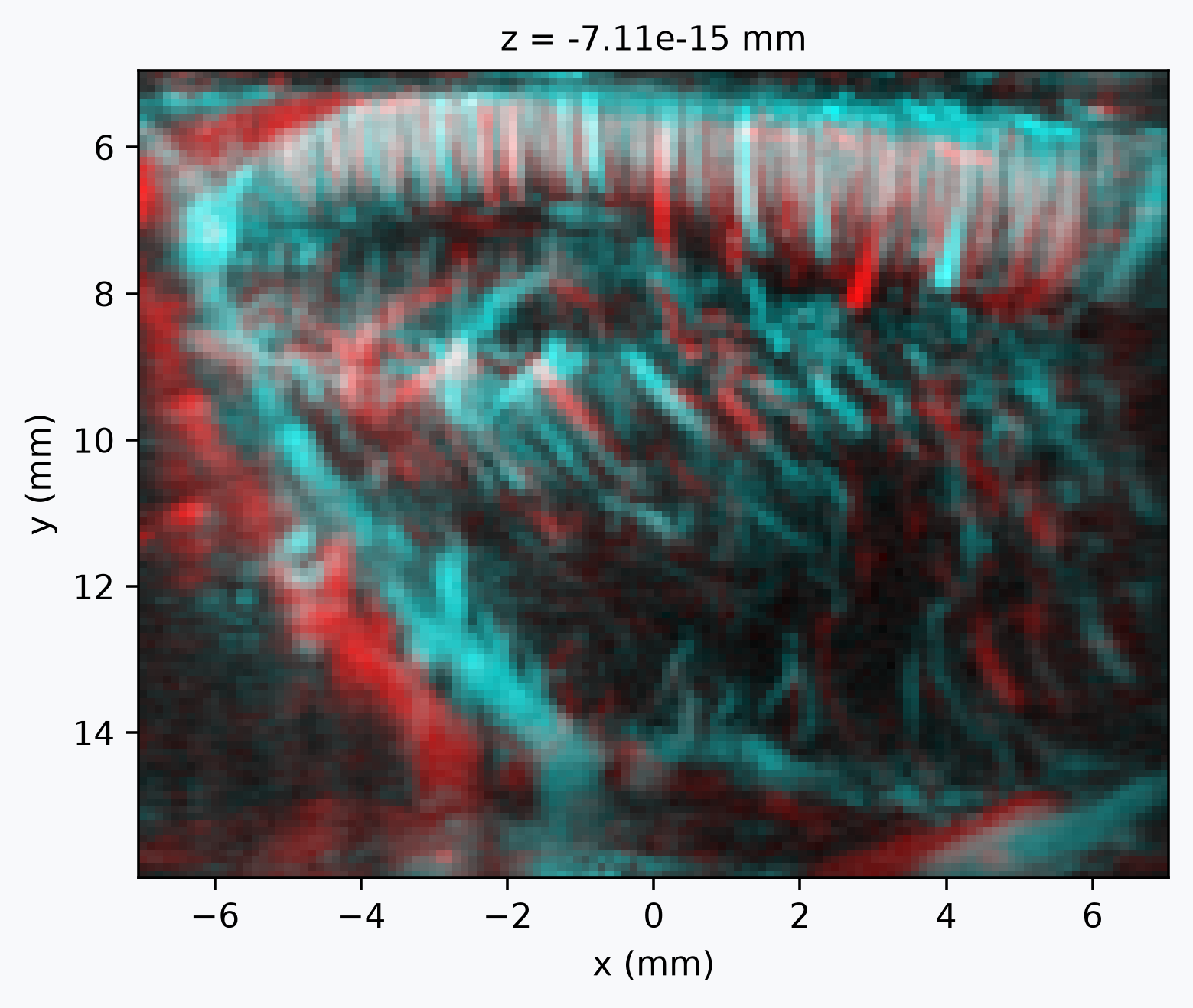
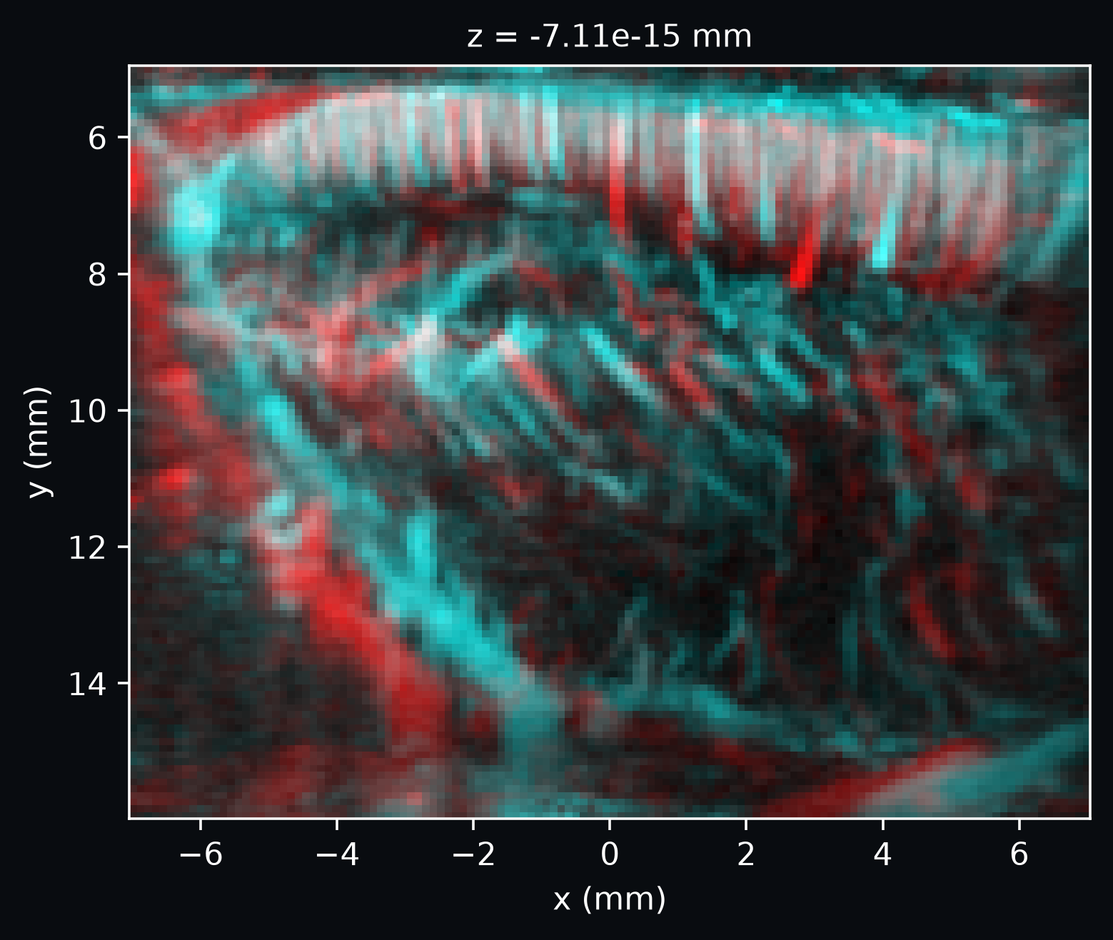
We visualize the alignment with
plot_composite, which resamples moving onto
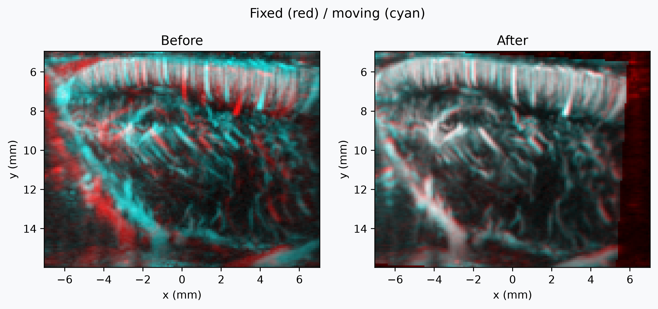
fixed's grid and draws the two as a red/cyan composite: matched anatomy appear in
white, while any residual red/cyan fringe reveals the displacement that
register_volume will correct.
Run the registration
A rigid transform captures the rotation and translation difference between the two
sessions. register_volume returns three
values:
- the moving image (only aligned to the fixed grid if
resample=Trueis used); - the rigid transform matrix that maps fixed-physical coordinates to moving-physical coordinates;
- a
RegistrationDiagnosticsdataclass holding the per-iteration metric values and the optimizer stop condition, which we use below to plot the convergence curve.
Watch registration progress live
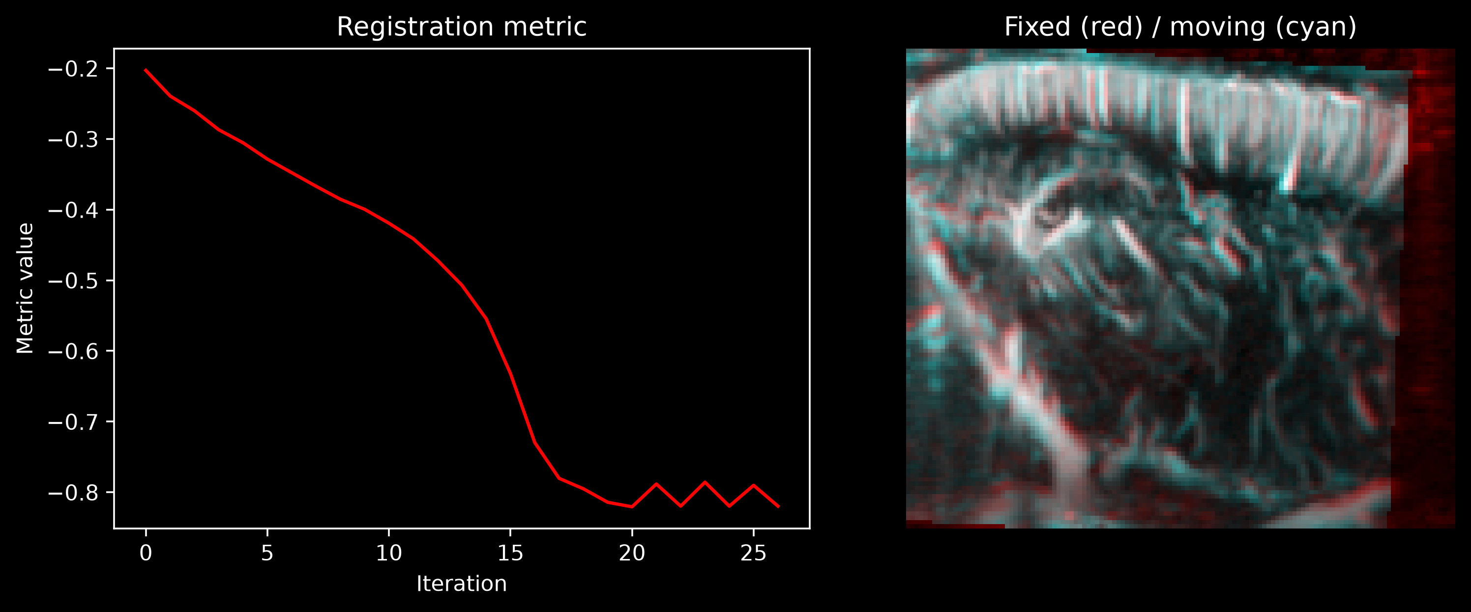
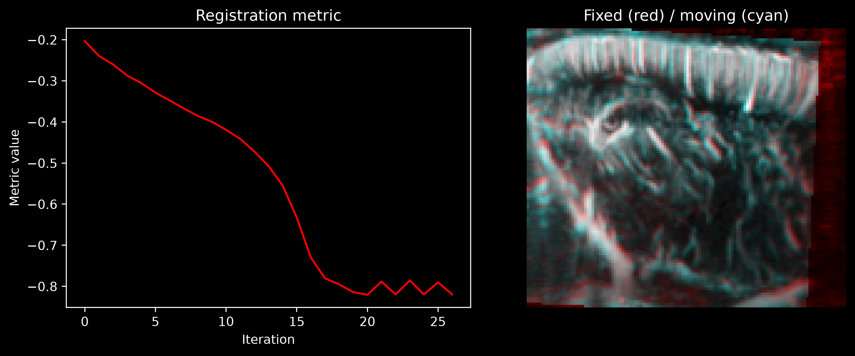
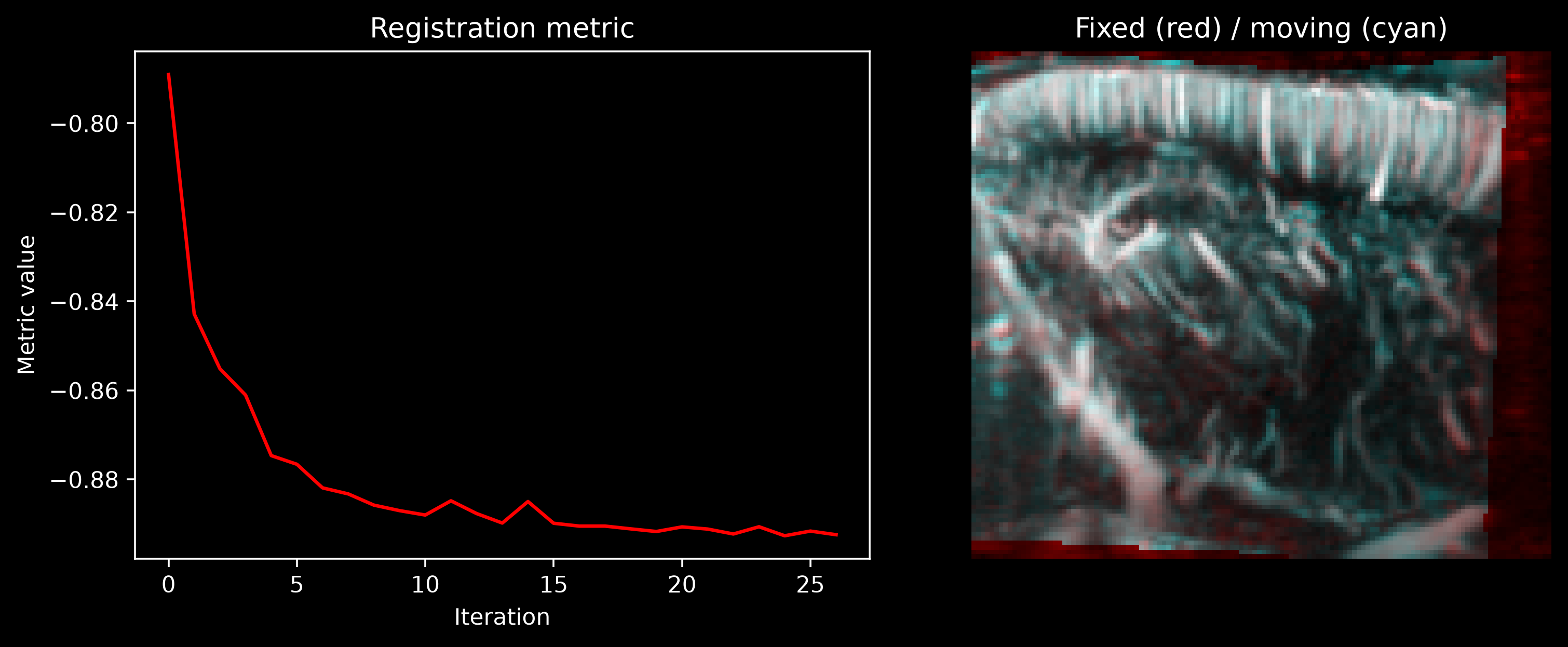
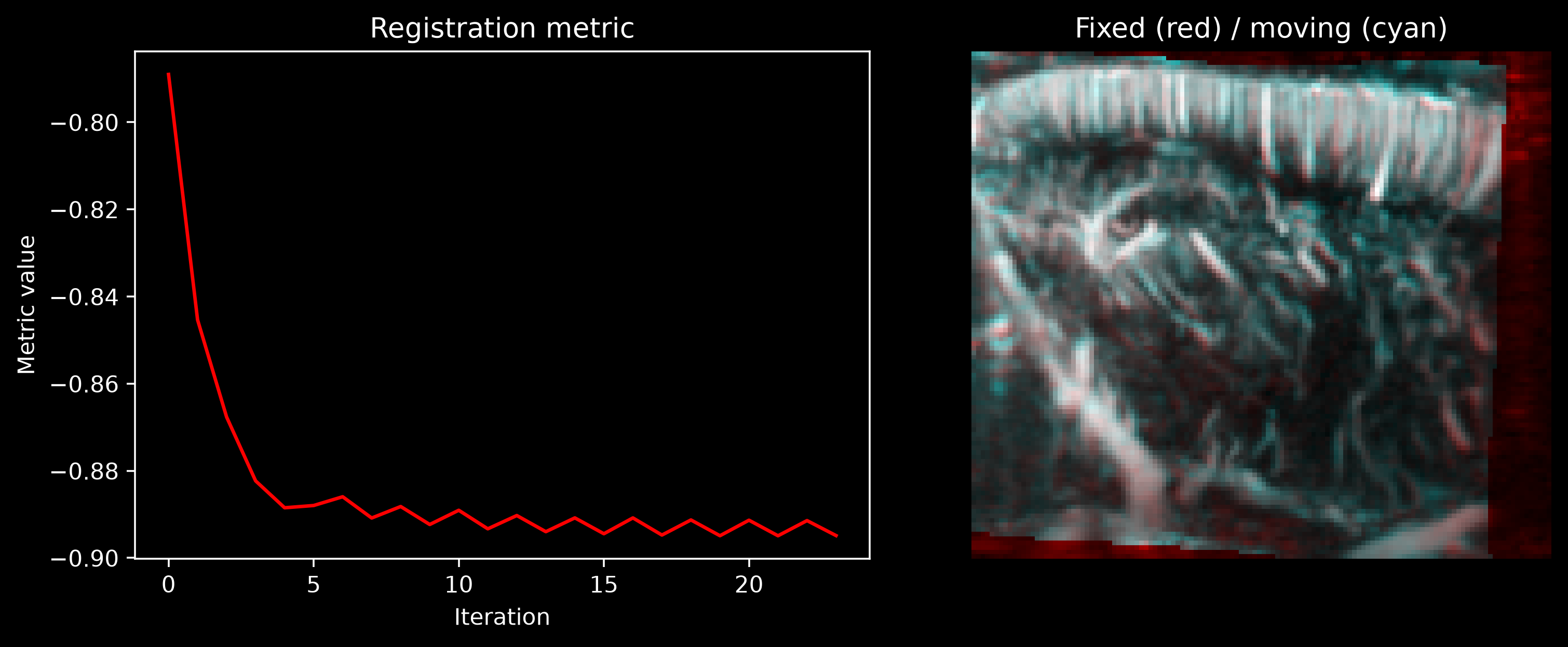
Pass show_progress=True to
register_volume to follow the
optimization in real time. A live matplotlib window opens during the call and
updates at every iteration with both the similarity-metric curve and a
fixed/moving composite overlay. It is the fastest way to tell whether the
optimizer is making progress, stuck in a local minimum, or diverging—and to
decide which arguments to tweak from the warning above.
Registration is sensitive to its arguments
The result depends heavily on the choice of transform_type, metric,
learning_rate, number_of_iterations, convergence_window_size,
initialization, and the multi-resolution settings (use_multi_resolution,
shrink_factors, smoothing_sigmas). The default values are usually a good
starting point and work well in many cases, but you should definitely try
different arguments (start with the default!). If the result is not satisfactory,
inspect the
RegistrationDiagnostics
convergence curve and the post-registration overlay, and sweep these arguments
until you get a stable, well-converged result.
registered, rigid_transform, diagnostics = cf.registration.register_volume(
    moving=moving, fixed=fixed, transform_type="rigid", show_progress=True
)
print(f"Rigid transform:\n{rigid_transform}")
Check the alignment after registration
Plotting the same fixed/moving overlay before and after registration makes the correction obvious: the red/cyan fringe in the first panel should be replaced by a more uniformly desaturated gray in the second.
fig, axes = plt.subplots(1, 2, figsize=(10, 4))
fig.patch.set_facecolor(bg_color)

for ax, moving_view, title in [
    (axes[0], moving, "Before"),
    (axes[1], registered, "After"),
]:
    cf.plotting.plot_composite(fixed, moving_view, axes=ax, bg_color=bg_color)
    ax.set_title(title)

_ = fig.suptitle("Fixed (red) / moving (cyan)")
Inspect convergence with the registration diagnostics
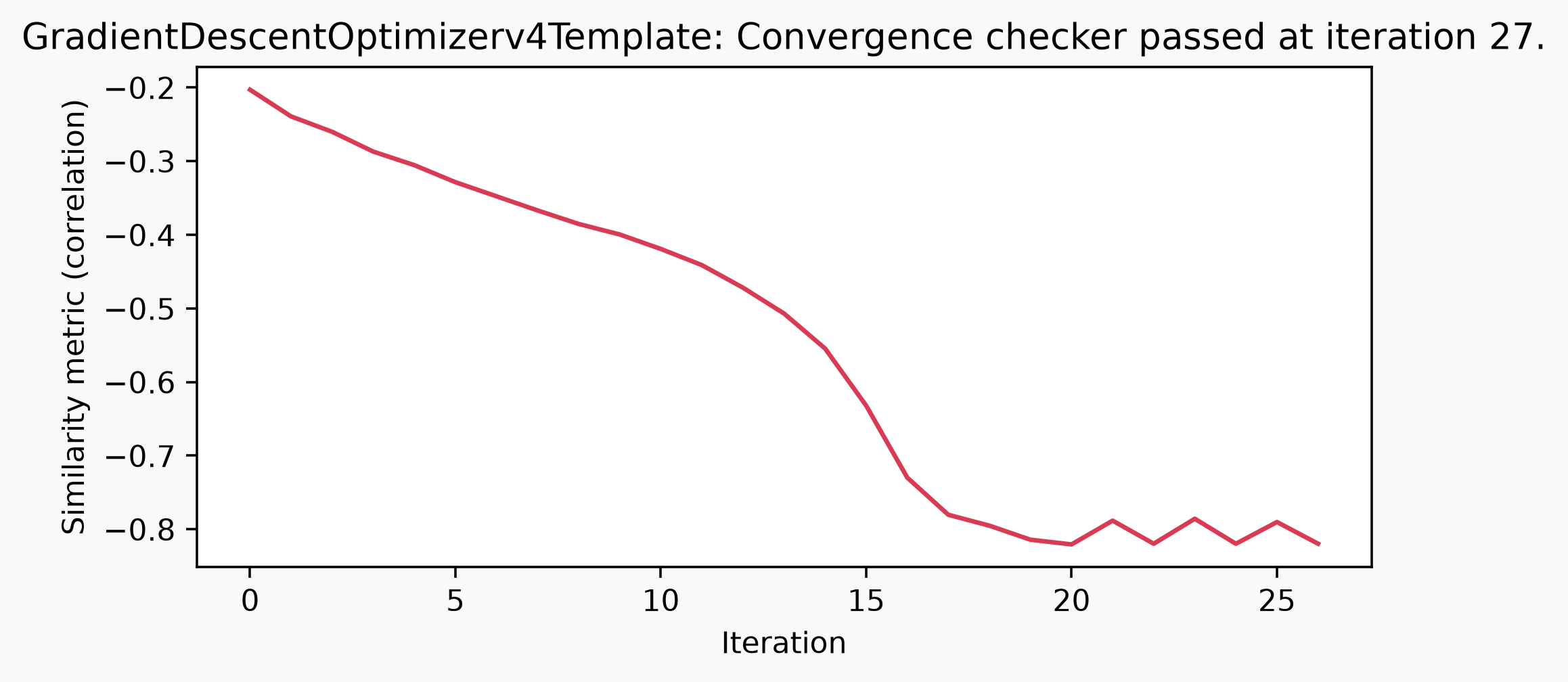
diagnostics.metric_values holds the optimizer's similarity-metric value at each
iteration. With the default metric="correlation", SimpleITK minimizes the negative
normalized cross-correlation, so a lower (more negative) value means a better fit.
The curve typically drops sharply at the start and then plateaus.
fig, ax = plt.subplots(figsize=(7, 3))
fig.patch.set_facecolor(bg_color)
ax.plot(diagnostics.metric_values, color="#d93a54")
ax.set_xlabel("Iteration")
ax.set_ylabel(f"Similarity metric ({diagnostics.metric})")
_ = ax.set_title(diagnostics.stop_condition)
The resulting rigid transform is encoded in physical units and can be reused, composed
with other transforms, or applied to additional volumes from the same session with
resample_volume.
Refine with a B-spline transform
A rigid transform only models a single global rotation and translation. Any residual
local mismatch—e.g. small elastic tissue deformation between sessions—needs a
nonrigid model. register_volume with
transform_type="bspline" fits a local displacement field on top of an initial
transform, here the rigid transform found above.
B-spline registration may need different parameters than rigid
Successful non-linear registration is often very dependent on the choice of
parameters. If the B-spline fails to converge, or if deformations are unrealistic,
try adjusting the learning_rate, mesh_size, and multi-resolution settings. The
default values are usually a good starting point, but you may need to experiment
to find the right combination for your data. Here, we use a non-default mesh size
of (6, 6, 6) to allow less local deformations that the default (10, 10, 10)
mesh would allow.
registered_bspline, bspline_transform, diagnostics_bspline = (
    cf.registration.register_volume(
        moving=moving,
        fixed=fixed,
        transform_type="bspline",
        mesh_size=(6, 6, 6),
        initialization=rigid_transform,
        show_progress=True,
    )
)
bspline_transform
- component: 3
- z: 9
- y: 9
- x: 9
- 1.616e-12 1.104e-13 4.067e-14 4.432e-14 ... -321.4 -108.7 -10.12
array([[[[ 1.61642547e-12, 1.10365432e-13, 4.06653554e-14, ..., 7.87230817e-14, 2.78266752e-13, -1.84752242e-09], [ 2.06768054e-13, 1.70067154e-14, 8.26192768e-15, ..., -1.19612270e-14, -5.48893708e-14, -3.23741293e-13], [ 5.03287565e-13, 3.66537400e-14, 1.07628688e-14, ..., -8.76788957e-15, -9.35552041e-15, -1.33548410e-14], ..., [ 2.57494295e-14, 1.89130561e-15, -2.31396304e-15, ..., -2.07198553e-15, -5.82140463e-15, -1.60475485e-15], [-2.33273808e-13, -2.17582914e-14, -8.56311095e-15, ..., 1.67159496e-15, -3.42026061e-15, -2.87727769e-15], [-2.87785513e-12, -2.41600934e-13, -5.99232128e-14, ..., -6.03587941e-15, -2.32166540e-14, -2.59763326e-14]], [[ 1.89415450e-15, 1.29328066e-16, 4.76523460e-17, ..., 9.22490285e-17, 3.26077652e-16, -2.16495888e-12], [ 2.42294276e-16, 1.99287546e-17, 9.68146553e-18, ..., -1.40163666e-17, -6.43202860e-17, -3.79365482e-16], [ 5.89760817e-16, 4.29514678e-17, 1.26121104e-17, ..., -1.02743602e-17, -1.09629558e-17, -1.56494268e-17], ... -9.21978471e-02, -1.23747411e-01, -7.31303576e-03], [ 1.49696294e-02, 5.35410574e-02, 1.30979303e-01, ..., -8.75539721e-02, -4.15487513e-02, -5.38484450e-03], [ 5.61298684e-02, 3.12561898e-01, 1.35632326e-01, ..., -3.76657451e-01, -1.27371564e-01, -1.18635198e-02]], [[ 8.93622931e+03, 6.56480773e+02, -3.75790870e+02, ..., -3.37703503e+02, -9.94726626e+00, 1.05116437e+01], [-5.01655074e+01, -1.88987729e+00, -7.83301436e+01, ..., -7.33103528e+01, 2.81280415e+00, 7.44817667e+00], [-4.78913984e+02, 5.99754364e+01, 3.73551654e+01, ..., -1.13928816e+02, 4.33762005e+00, 5.78823312e+00], ..., [-4.49817021e+01, 1.03353656e+02, 1.87733948e+02, ..., -7.86794048e+01, -1.05603037e+02, -6.24076719e+00], [ 1.27747184e+01, 4.56906388e+01, 1.11774558e+02, ..., -7.47164345e+01, -3.54566958e+01, -4.59529562e+00], [ 4.78998686e+01, 2.66732734e+02, 1.15745334e+02, ..., -3.21430326e+02, -1.08695801e+02, -1.01240397e+01]]]], shape=(3, 9, 9, 9)) - component(component)<U1'z' 'y' 'x'
array(['z', 'y', 'x'], dtype='<U1')
- z(z)float64-0.2833 -0.2125 ... 0.2125 0.2833
array([-0.283333, -0.2125 , -0.141667, -0.070833, 0. , 0.070833, 0.141667, 0.2125 , 0.283333]) - y(y)float643.095 4.938 6.782 ... 16.0 17.85
array([ 3.094506, 4.9384 , 6.782293, 8.626187, 10.47008 , 12.313973, 14.157867, 16.00176 , 17.845653]) - x(x)float64-9.405 -7.054 ... 7.054 9.405
array([-9.405000e+00, -7.053750e+00, -4.702500e+00, -2.351250e+00,
        4.768372e-07,  2.351250e+00,  4.702501e+00,  7.053751e+00,
        9.405001e+00])
- transform_type :
- bspline_transform
- order :
- 3
- direction :
- [[1.0, 0.0, 0.0], [0.0, 1.0, 0.0], [0.0, 0.0, 1.0]]
- affines :
- {'bspline_initialization': [[1.0, 9.95283452360052e-21, -4.41182359981892e-21, 7.105323150629779e-15], [-1.0180748365323002e-20, 0.9984816653136261, -0.05508506179108773, -0.1770895799666997], [3.856872470288146e-21, 0.05508506179108773, 0.9984816653136261, 0.8544666816293863], [0.0, 0.0, 0.0, 1.0]]}
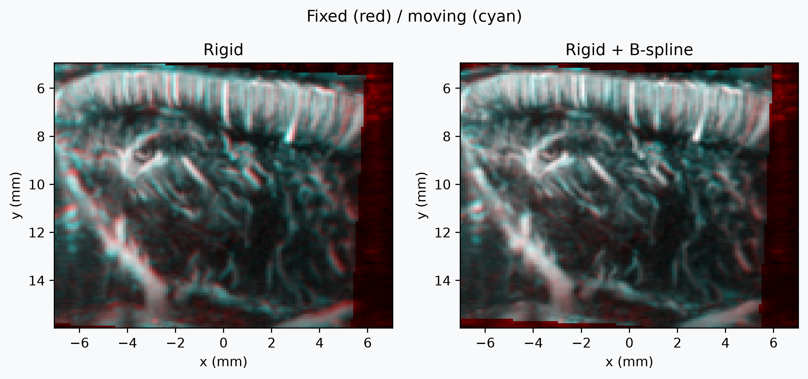
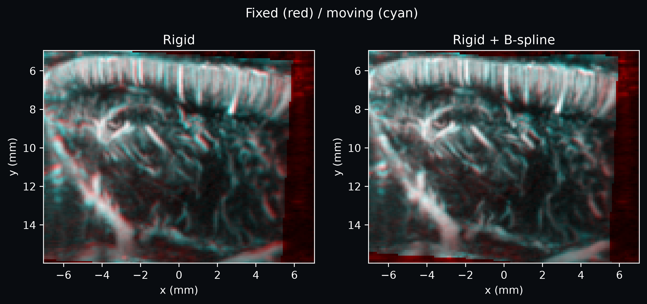
Check the alignment after B-spline refinement
Comparing the rigid-only result against the B-spline-refined result shows the extra local correction the B-spline step adds on top of rigid, especially in deeper vessels where the brain might have contracted slightly between sessions.
print(f"Rigid final metric: {diagnostics.final_metric_value:.4f}")
print(f"Rigid + B-spline final metric: {diagnostics_bspline.final_metric_value:.4f}")
fig, axes = plt.subplots(1, 2, figsize=(10, 4))
fig.patch.set_facecolor(bg_color)

for ax, moving_view, title in [
    (axes[0], registered, "Rigid"),
    (axes[1], registered_bspline, "Rigid + B-spline"),
]:
    cf.plotting.plot_composite(fixed, moving_view, axes=ax, bg_color=bg_color)
    ax.set_title(title)

_ = fig.suptitle("Fixed (red) / moving (cyan)")
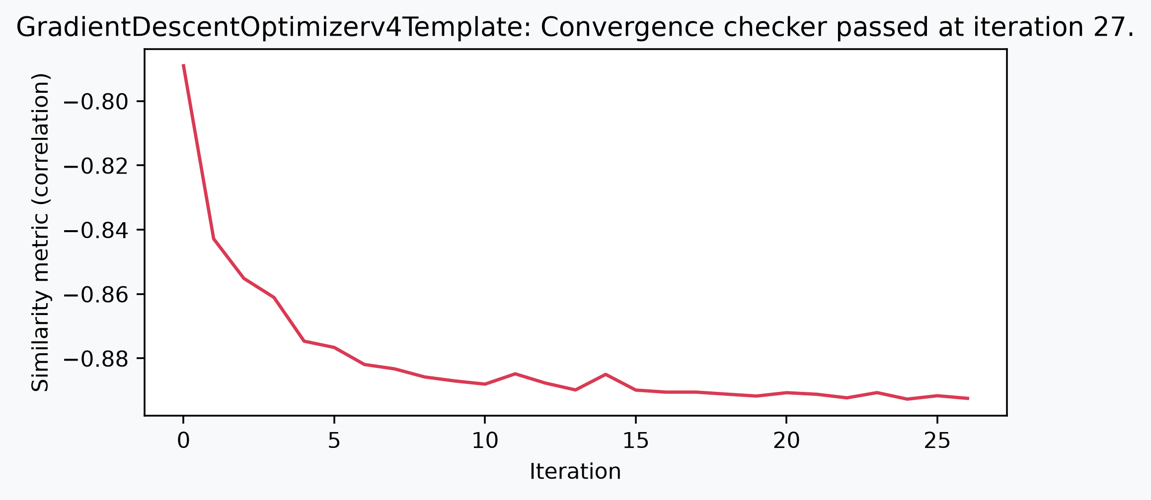
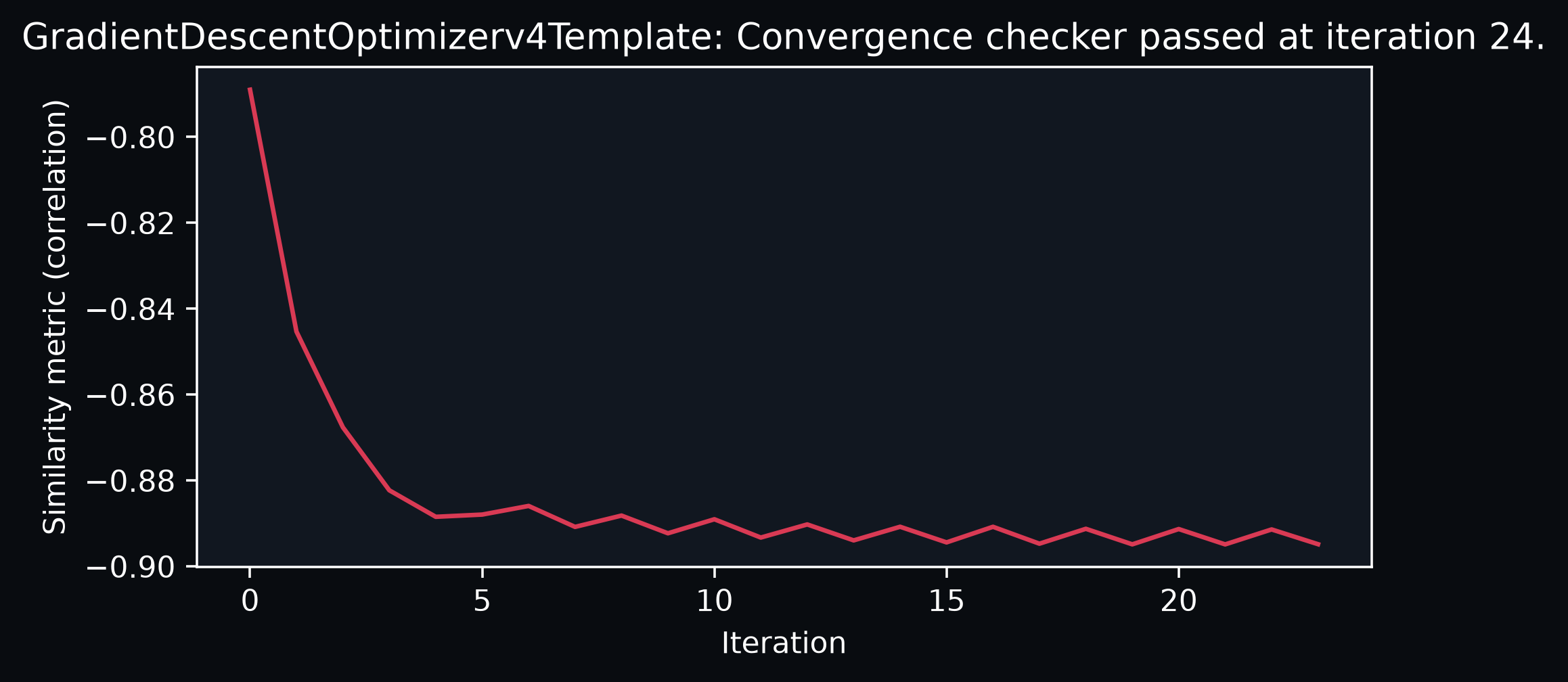
Inspect B-spline convergence
fig, ax = plt.subplots(figsize=(7, 3))
fig.patch.set_facecolor(bg_color)
ax.plot(diagnostics_bspline.metric_values, color="#d93a54")
ax.set_xlabel("Iteration")
ax.set_ylabel(f"Similarity metric ({diagnostics_bspline.metric})")
_ = ax.set_title(diagnostics_bspline.stop_condition)
Visualize the deformation
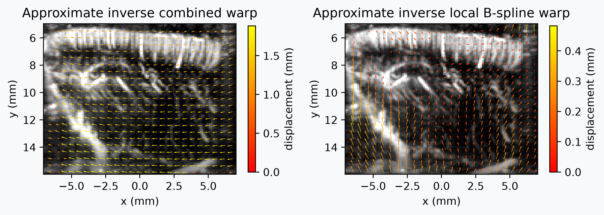
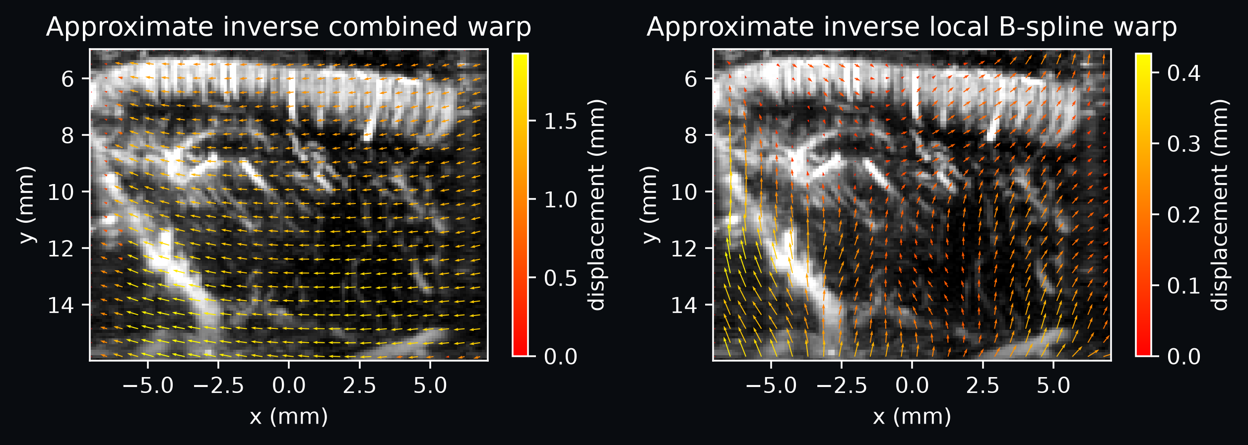
To see the deformation directly, sample the B-spline transform onto fixed's grid
with
sample_displacement_field_like,
which returns one displacement vector per voxel of the reference grid.
Sampling bspline_transform includes the rigid pre-affine it was initialized with,
giving the combined rigid + B-spline warp; dropping that pre-affine leaves only the
local B-spline deformation.
The sampled field follows the pull convention (fixed-to-moving): at each fixed-grid
point it indicates where to look in moving. That is correct for warping, but less
intuitive to read as motion, so for the figure below we invert the field and plot the
approximate moving-to-fixed displacement instead. The inverse is only approximate,
because a B-spline transform has no closed-form inverse and must be inverted through
its sampled displacement field.
# Combined rigid + B-spline field.
composite_field = cf.registration.sample_displacement_field_like(
    bspline_transform, fixed
)

# Local-only field: copy the transform and drop the rigid pre-affine before sampling.
local_bspline = bspline_transform.copy()
local_bspline.attrs = {**local_bspline.attrs, "affines": {}}
local_field = cf.registration.sample_displacement_field_like(local_bspline, fixed)

# For display, invert the pull fields so the arrows show apparent motion toward
# `fixed`, rather than the fixed-to-moving lookup direction SimpleITK uses for
# resampling.
composite_inverse_field = cf.registration.invert_displacement_field(composite_field)
local_inverse_field = cf.registration.invert_displacement_field(local_field)
A quiver plot draws the in-plane displacement as arrows over the anatomy, so the
direction of the warp is easy to read. The field carries a leading component axis
labeled by the spatial dim names, so we use the x and y displacement components,
drop the degenerate z of the single slice, and subsample the dense grid so the
arrows stay legible.
fig, axes = plt.subplots(1, 2, figsize=(8, 3))
fig.patch.set_facecolor(bg_color)

for ax, background, field, title in [
    (axes[0], fixed, composite_inverse_field, "Approximate inverse combined warp"),
    (axes[1], fixed, local_inverse_field, "Approximate inverse local B-spline warp"),
]:
    cf.plotting.plot_volume(background, axes=ax, show_colorbar=False, bg_color=bg_color)
    # x- and y-displacement of the single slice.
    disp_x = field.sel(component="x").squeeze(drop=True)
    disp_y = field.sel(component="y").squeeze(drop=True)
    # Subsample to roughly 20 arrows along the shorter axis so the field stays readable.
    step = max(1, min(disp_x.sizes["y"], disp_x.sizes["x"]) // 20)
    grid_x, grid_y = np.meshgrid(disp_x["x"].values[::step], disp_x["y"].values[::step])
    u = disp_x.values[::step, ::step]
    v = disp_y.values[::step, ::step]
    arrows = ax.quiver(grid_x, grid_y, u, v, np.hypot(u, v), angles="xy", cmap="autumn")
    fig.colorbar(arrows, ax=ax, label="displacement (mm)", shrink=0.75)
    ax.set_aspect("equal")
    ax.set_title(title)
    ax.set_xlabel("x (mm)")
    ax.set_ylabel("y (mm)")

# Arrow lengths are autoscaled per panel, so compare directions and patterns, not
# absolute length between the two.
fig.tight_layout()
Total running time: 57.8 s