Searchlight decoding of a continuous variable¶

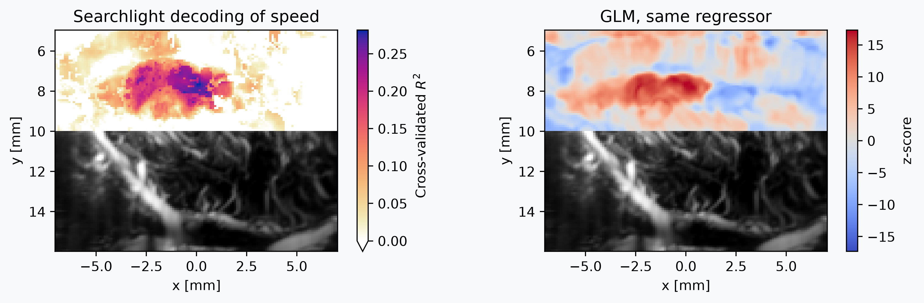
This example maps which parts of a fUSI recording carry information about how fast a rat is moving with a searchlight: a small cross-validated model run over the local neighborhood of every voxel. Unlike a GLM, which asks voxel by voxel whether one voxel's signal tracks the regressor, the searchlight asks whether the local pattern around each voxel can predict it, picking up information carried jointly by neighboring voxels rather than by any one alone.

We follow the experimental setting and dataset of Cybis Pereira et al. 2026, decoding locomotion speed from a single sagittal plane, and compare the searchlight map against a GLM fit on the same data. Both analyses receive the same preprocessing steps, so the only thing that differs between them is univariate versus multivariate, which is the comparison we actually want to make.

Load the recording and the tracking data¶

from functools import partial
from pathlib import Path

import colorcet as cc
import matplotlib as mpl
import matplotlib.pyplot as plt
import numpy as np
import pandas as pd
import xarray as xr
from sklearn.linear_model import RidgeCV

import confusius as cf

# Adapt background color to the current Matplotlib style.
bg_color = mpl.colors.to_hex(mpl.rcParams["figure.facecolor"])

xr.set_options(display_expand_data=False)

subject = "rat75"
session = "20220524"
acq = "slice32"


bids_root = cf.datasets.fetch_cybis_pereira_2026(
    datasets="rawdata",
    subjects=subject,
    sessions=session,
    acqs=acq,
)

session_dir = Path(bids_root) / f"sub-{subject}" / f"ses-{session}"
stem = f"sub-{subject}_ses-{session}_task-openfield"

pwd_path = session_dir / "fusi" / f"{stem}_acq-{acq}_pwd.nii.gz"
motion_path = session_dir / "motion" / f"{stem}_tracksys-DLC_acq-{acq}_motion.tsv"

data = cf.load(pwd_path).compute()
data

If you use this dataset in your work, please cite the following source:

Cybis Pereira, F., Castedo, S. H., Meur-Diebolt, S. L., Ialy-Radio, N., Bhattacharya, S., Ferrier, J., Osmanski, B.
F., Cocco, S., Monasson, R., Pezet, S., & Tanter, M. (2026). A vascular code for speed in the spatial navigation 
system. Cell Reports, 45(1). https://doi.org/10.1016/j.celrep.2025.116791

Correct for motion¶

The rat moves freely, so a real analysis should first correct volume-to-volume brain motion. We skip it here to keep the example fast to build, at the cost of a little statistical robustness in the maps below.

data = cf.registration.register_volumewise(data, learning_rate=1)

Build the speed regressor¶

The animal is tracked with DeepLabCut at 50 frames per second. We take the frame-to-frame displacement of the body marker, smooth it with a one second centered rolling mean, and resample it onto the fUSI volume acquisition times.

fps = 50
motion_df = pd.read_csv(motion_path, sep="\t")
squared_diff = motion_df[["body_x", "body_y"]].diff() ** 2
speed_df = fps * (squared_diff["body_x"] + squared_diff["body_y"]) ** 0.5
speed_df[0] = 0
speed = (
    xr.DataArray(
        speed_df,
        dims=["time"],
        coords={"time": 1 / fps * np.arange(len(speed_df))},
        name="speed",
    )
    .rolling(time=fps, min_periods=1, center=True)
    .mean()
)
speed = speed.interp(time=data.time, method="linear").ffill("time")

What the searchlight should actually predict¶

The speed signal above is an instantaneous behavioral variable, and the power Doppler signal contains a proxy of the neural signal encoding the speed signal through the neurovascular coupling. With the neurovascular coupling inherent delay, asking a decoder to predict the instantaneous trace from that signal sets it an impossible target. We therefore decode an hemodynamically convolved speed regressor.

We build it with the modified Claron 2021 HRF, a rodent fUSI response function, and read it straight off a first-level design matrix. Building the design matrix here serves double duty: its speed column is the searchlight target, and the whole matrix is what we hand the GLM later, so the two analyses are guaranteed to see the same regressor.

modified_claron2021 = partial(cf.glm.claron2021_hrf, beta=6.7)

events = pd.DataFrame(
    {
        "onset": data.time.values,
        "duration": data.time.volume_acquisition_duration,
        "modulation": speed.values,
        "trial_type": "speed",
    }
)
confounds = cf.signal.compute_compcor_confounds(
    data,
    variance_threshold=0.05,
    n_components=3,
)


design_matrix = cf.glm.make_first_level_design_matrix(
    data.time.values,
    events=events,
    hrf_model=modified_claron2021,
    drift_model="cosine",
    low_cutoff=0.01,
    confounds=confounds,
)

The speed column of the design matrix is the raw speed trace convolved with the HRF. We read it out as the searchlight target.

speed_regressor = design_matrix["speed"].to_numpy()

Preprocess the data exactly as the GLM does¶

The point of this example is to compare a univariate analysis with a multivariate one, which only works if everything else is held equal. So the decoder gets the same preprocessing the GLM applies.

Spatial smoothing. FirstLevelModel(smoothing_fwhm=0.3) smooths each run with smooth_volume before fitting. We apply the same call with the same value, rather than leaving the searchlight to work on unsmoothed data while the GLM enjoys the noise reduction.

Drift and confound removal. Power Doppler carries slow drift and nuisance signal that have nothing to do with locomotion. The GLM handles them with cosine drift and CompCor regressors in its design; a decoder has no design matrix, so we remove the same regressors from the data up front with clean, reusing the design matrix's own nuisance columns.

The target is cleaned with the same regressors as the data, so both sides have the same nuisance structure removed. This mirrors what the GLM does implicitly when it fits the speed regressor and the nuisance regressors jointly.

smoothing_fwhm = 0.3

confounds_np = design_matrix.drop(columns="speed").to_numpy()
confounds = xr.DataArray(
    confounds_np, dims=["time", "confound"], coords={"time": data.time}
)


cleaned = cf.signal.clean(
    cf.spatial.smooth_volume(data, smoothing_fwhm),
    standardize_method="zscore",
    confounds=confounds,
)
target = cf.signal.clean(
    xr.DataArray(
        speed_regressor, dims=["time"], coords={"time": data.time}, name="speed"
    ),
    standardize_method="zscore",
    confounds=confounds,
)

Run the searchlight¶

Running searchlight through the entire field of view is costly because this means fitting a few tens of thousands of models. Here we will create a mask to only run the searchlight algorithm in the top half of the field of view. A real region-of-interest mask, such as an intensity-thresholded brain mask, or an anatomical brain region mask, would be of good use here just the same.

Two details matter for fUSI data:

• radius is in the units of the data's spatial coordinates, not in voxel indices. Each neighborhood is the set of voxels within radius millimeters of the center.
• Consecutive fUSI volumes are strongly autocorrelated. Cross-validating with shuffled folds would put near-duplicate volumes in both the training and test sets and inflate the scores. SearchLight therefore builds contiguous temporal folds by default. Each fold also needs to be long enough to contain both quiet and active periods, since the animal moves in bursts, which is why we keep the fold count low.

The estimator is a RidgeCV: ridge regression that selects its own penalty from a grid. Neighboring fUSI voxels are highly correlated, and the right amount of regularization varies across the plane. By default RidgeCV picks the penalty by leave-one-out generalized cross-validation, which does put temporally adjacent volumes in its train and test sets, unlike the contiguous folds we use for the outer searchlight cross-validation. That is not a problem: the penalty search runs entirely inside each outer training fold and never sees the outer test fold, so it only affects which penalty is chosen.

estimator = RidgeCV(alphas=np.logspace(0, 10, 5))
mask = xr.ones_like(cleaned.isel(time=0), dtype=bool).where(cleaned.y < 10, False)

searchlight = cf.decoding.SearchLight(
    estimator=estimator, mask=mask, radius=0.6, cv=3, n_jobs=-1
)
searchlight.fit(cleaned, target.values)
searchlight.scores_

Compare against a GLM¶

We now fit a GLM with the design matrix built earlier, so it tests the same HRF-convolved speed regressor against the same drift model, on data smoothed with the same kernel.

glm = cf.glm.FirstLevelModel(smoothing_fwhm=smoothing_fwhm)
glm.fit(data, design_matrices=design_matrix)
z_scores = glm.compute_contrast("speed")

Compare the two maps¶

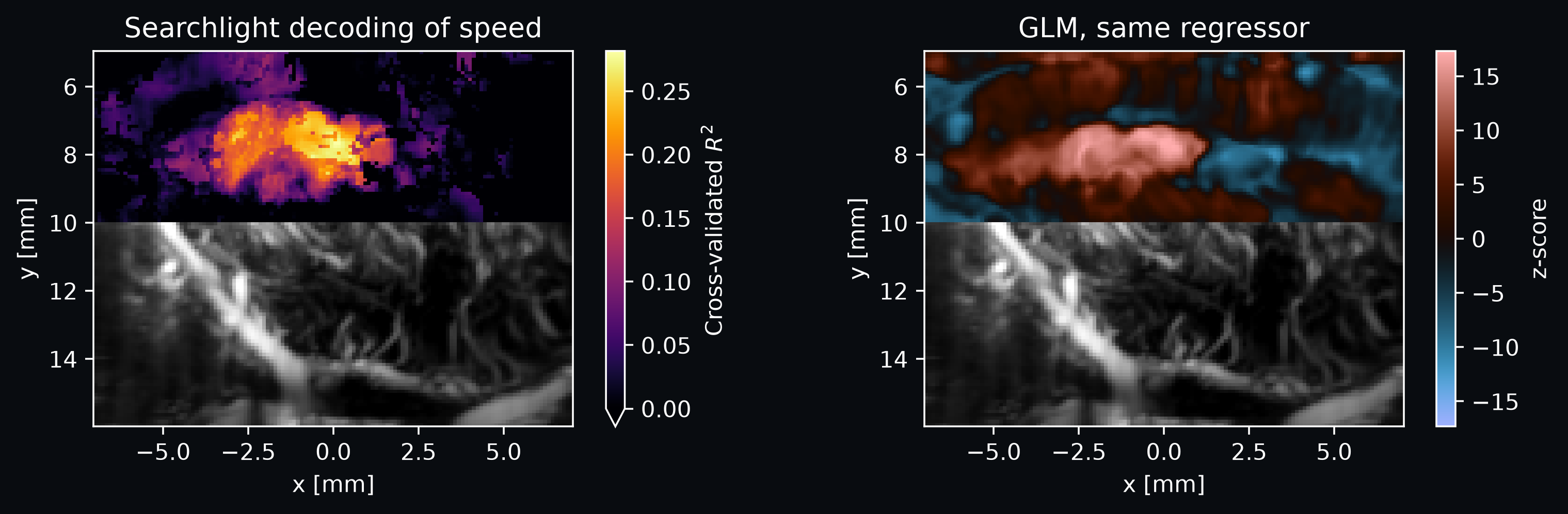
The searchlight reports a cross-validated coefficient of determination, so values at or below zero mean the local neighborhood predicts the speed regressor no better than the fold mean; we clip the color scale at zero. The GLM reports a z-score for the speed contrast. Both maps cover the whole plane.

is_dark_theme = sum(mpl.colors.to_rgb(bg_color)) / 3 < 0.5
searchlight_cmap = "inferno" if is_dark_theme else cc.cm.CET_L17
glm_cmap = "berlin" if is_dark_theme else "coolwarm"

background_data = data.mean("time").fusi.scale.db()

fig, axes = plt.subplots(1, 2, figsize=(10, 3), constrained_layout=True)

background_data.fusi.plot.volume(axes=axes[0], show_colorbar=False, bg_color=bg_color)
searchlight.scores_.plot(
    ax=axes[0],
    cmap=searchlight_cmap,
    vmin=0,
    cbar_kwargs={"label": "Cross-validated $R^2$"},
)
axes[0].set_title("Searchlight decoding of speed")

background_data.fusi.plot.volume(axes=axes[1], show_colorbar=False, bg_color=bg_color)
z_scores.where(mask).plot(
    ax=axes[1], cmap=glm_cmap, center=0, cbar_kwargs={"label": "z-score"}
)
axes[1].set_title("GLM, same regressor")

for ax in axes:
    ax.set_aspect("equal")
    ax.invert_yaxis()

We quantify the spatial agreement between the two maps by the Dice overlap of their top 5 percent of voxels.

top_scores = searchlight.scores_.squeeze(drop=True)
top_z = z_scores.squeeze(drop=True)

selected_scores = top_scores >= top_scores.quantile(0.95)
selected_z = top_z >= top_z.quantile(0.95)
dice = float(
    2
    * (selected_scores & selected_z).sum()
    / (selected_scores.sum() + selected_z.sum())
)
print(f"Top-5% overlap, Dice = {dice:.3f}")

Top-5% overlap, Dice = 0.462

The overlap is partial: the two maps answer related but different questions. The GLM is univariate and asks, at each voxel, whether that voxel's signal tracks the speed regressor. The searchlight is multivariate and cross-validated, and asks whether the local pattern around each voxel predicts the regressor in held-out blocks of time.

Total running time: 88.3 s

Launch in Binder Download .py Download .ipynb