Motion correction of a single recording¶

This example shows how to correct volume-to-volume brain motion in one fUSI recording with register_volumewise. For this example, we use a short subset of an open-field 2D+t recording from the Cybis Pereira 2026 dataset. After volumewise registration, we inspect three things that are useful in practice:

the motion diagnostics returned by create_motion_dataframe;
a representative voxel trace before and after registration;
a compact raster view showing how volumewise registration stabilized the recording.

Fetch and load a short motion-corrupted window¶

The selected acquisition is a recording from a single 2D slice, so the data shape is (time, z=1, y, x).

from pathlib import Path

import matplotlib as mpl
import matplotlib.pyplot as plt
import numpy as np
import xarray as xr

import confusius as cf

bg_color = mpl.colors.to_hex(mpl.rcParams["figure.facecolor"])
xr.set_options(display_expand_data=False)

subject = "rat75"
session = "20220523"
acq = "slice32"
start_frame = 220
n_frames = 120

bids_root = cf.datasets.fetch_cybis_pereira_2026(
    datasets="rawdata",
    subjects=subject,
    sessions=session,
    acqs=acq,
)

If you use this dataset in your work, please cite the following source:

Cybis Pereira, F., Castedo, S. H., Meur-Diebolt, S. L., Ialy-Radio, N., Bhattacharya, S., Ferrier, J., Osmanski, B.
F., Cocco, S., Monasson, R., Pezet, S., & Tanter, M. (2026). A vascular code for speed in the spatial navigation 
system. Cell Reports, 45(1). https://doi.org/10.1016/j.celrep.2025.116791

pwd_path = (
    Path(bids_root)
    / f"sub-{subject}"
    / f"ses-{session}"
    / "fusi"
    / f"sub-{subject}_ses-{session}_task-openfield_acq-{acq}_pwd.nii.gz"
)

data = cf.load(pwd_path).isel(time=slice(start_frame, start_frame + n_frames)).compute()
data

Register every frame to the first frame¶

Volumewise registration can be applied using register_volumewise. By default, each volume (or frame in this case) is registered to the first acquired volume. You may choose any other reference timepoint using the reference_time. Here, we're trying to correct for rigid motion—that is, translation and rotations. A learning rate of 1.0 leads to good convergence across frames.

registered = cf.registration.register_volumewise(
    data,
    transform="rigid",
    metric="correlation",
    learning_rate=1.0,
)

register_volumewise adds a motion_params attribute to the motion-corrected DataArray. motion_params is a DataFrame created using create_motion_dataframe and containing the motion parameters and registration diagnostics: rotations (rot_x, rot_y, rot_z), translations (trans_x, trans_y, trans_z), the framewise displacement (FD)¹ summaries (mean_fd, max_fd, rms_fd), and the optimizer summaries (final_metric_value, n_iterations) added by register_volumewise. Since we registered a 2D+t recording, only the rotation along the z-axis and the translations along the x- and y-axes are non-zero.

motion_df = registered.attrs["motion_params"]
motion_df.head()

	rot_x	rot_y	rot_z	trans_x	trans_y	trans_z	mean_fd	max_fd	rms_fd	final_metric_value	n_iterations	status
time
88.401400	0.000000e+00	-0.000000e+00	0.000000	0.000000	0.000000	0.000000e+00	0.008461	0.012281	0.008704	-1.000000	31	completed
88.801400	1.496784e-21	-6.225587e-21	0.000512	-0.005748	-0.008282	1.570482e-20	0.035006	0.043871	0.035202	-0.966427	31	completed
89.201400	-5.956531e-21	-2.754602e-21	0.001581	0.011977	-0.027575	-6.231969e-20	0.035979	0.052521	0.036672	-0.971177	33	completed
89.601425	-2.058074e-20	-1.901582e-21	0.003542	0.016896	-0.051908	-2.154101e-19	0.005747	0.007470	0.005799	-0.961348	31	completed
90.001425	-3.390010e-21	-1.791389e-21	0.003781	0.019862	-0.053373	-3.542251e-20	0.007024	0.007902	0.007034	-0.962170	35	completed

Plot the motion diagnostics¶

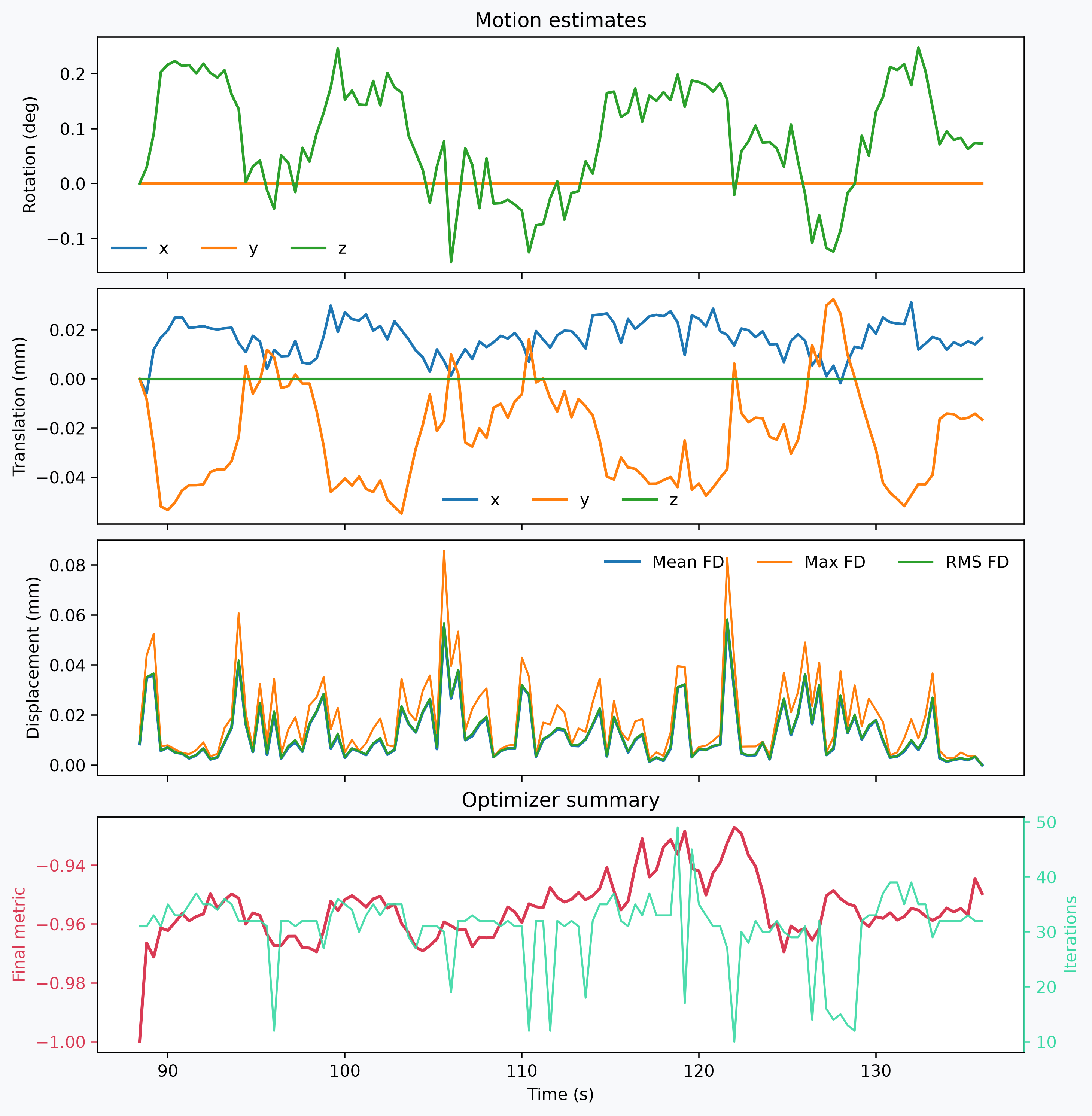
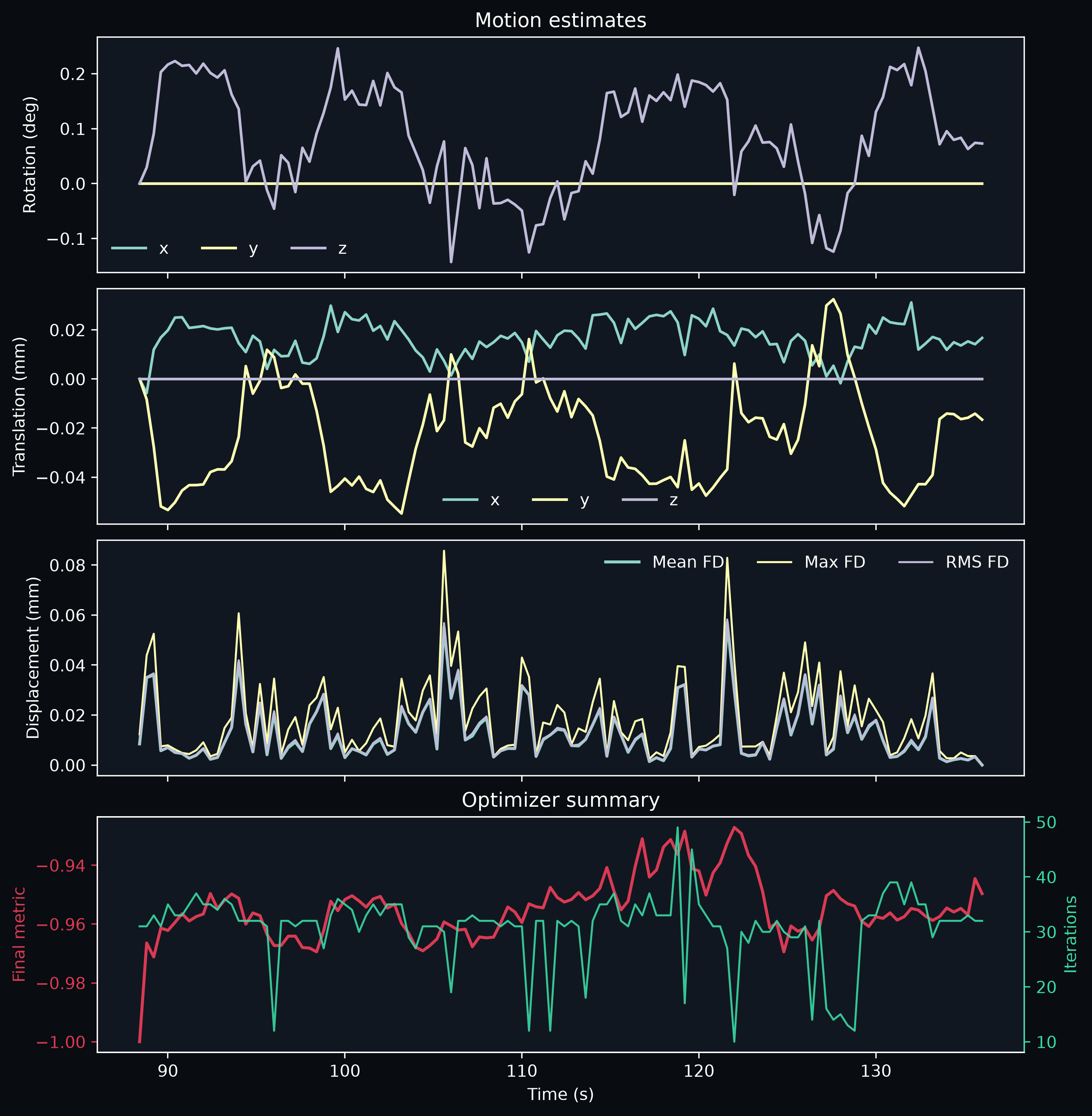
ConfUSIus provides the function plot_motion_diagnostics to plot motion_params using four panels:

The first two panels show the rotations and translations found at each frame.
The third panel shows the mean, maximum, and RMS of the framewise displacement (FD). The FD is a metric used to quantify brain motion between consecutive volumes by summing the absolute temporal derivatives of the realignment parameters (translations and rotations)¹.
The fourth panel shows the final registration metric and iteration count for each volume. Volumes showing outlier metric values or reaching the maximum number of iterations configured in register_volumewise are likely to not be registered correctly. In that case, you might want to tweak the registration parameters, or remove the corresponding volumes from further analysis.

fig, axes = cf.plotting.plot_motion_diagnostics(motion_df)
fig.patch.set_facecolor(bg_color)

Compare a representative time series before and after registration¶

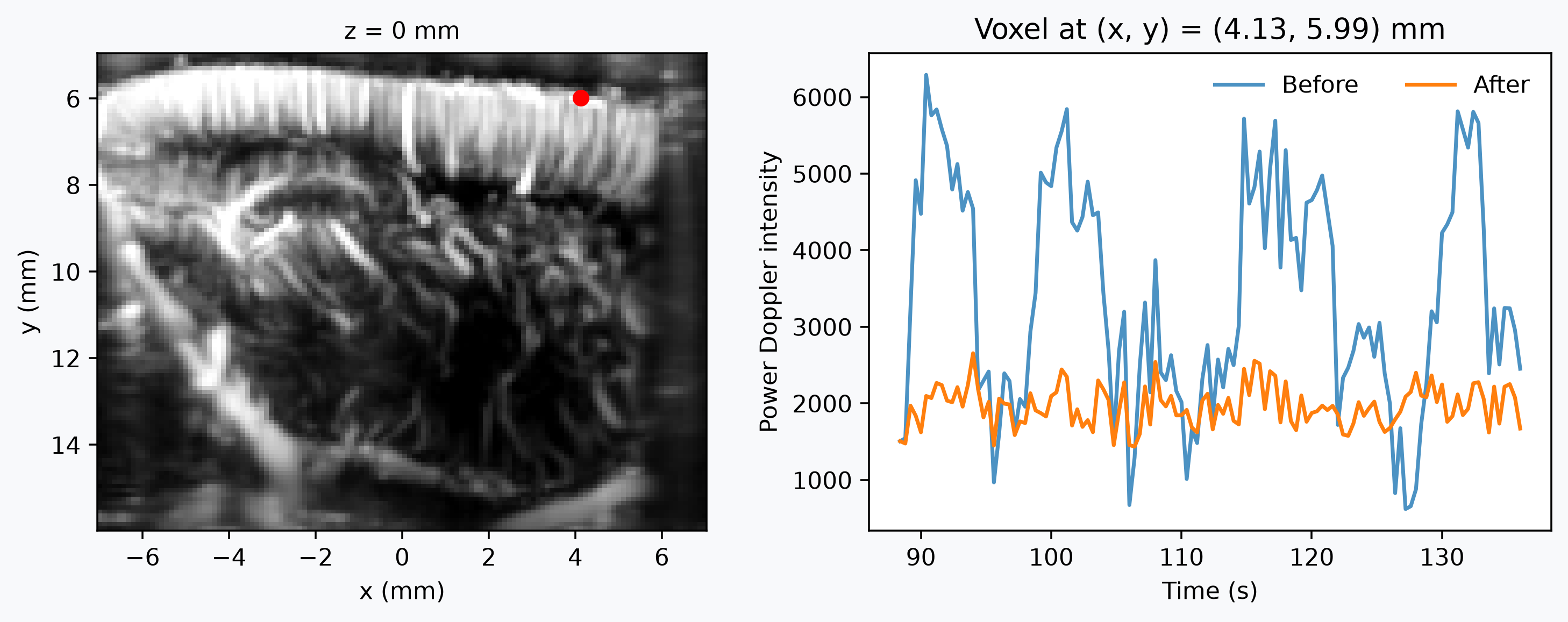
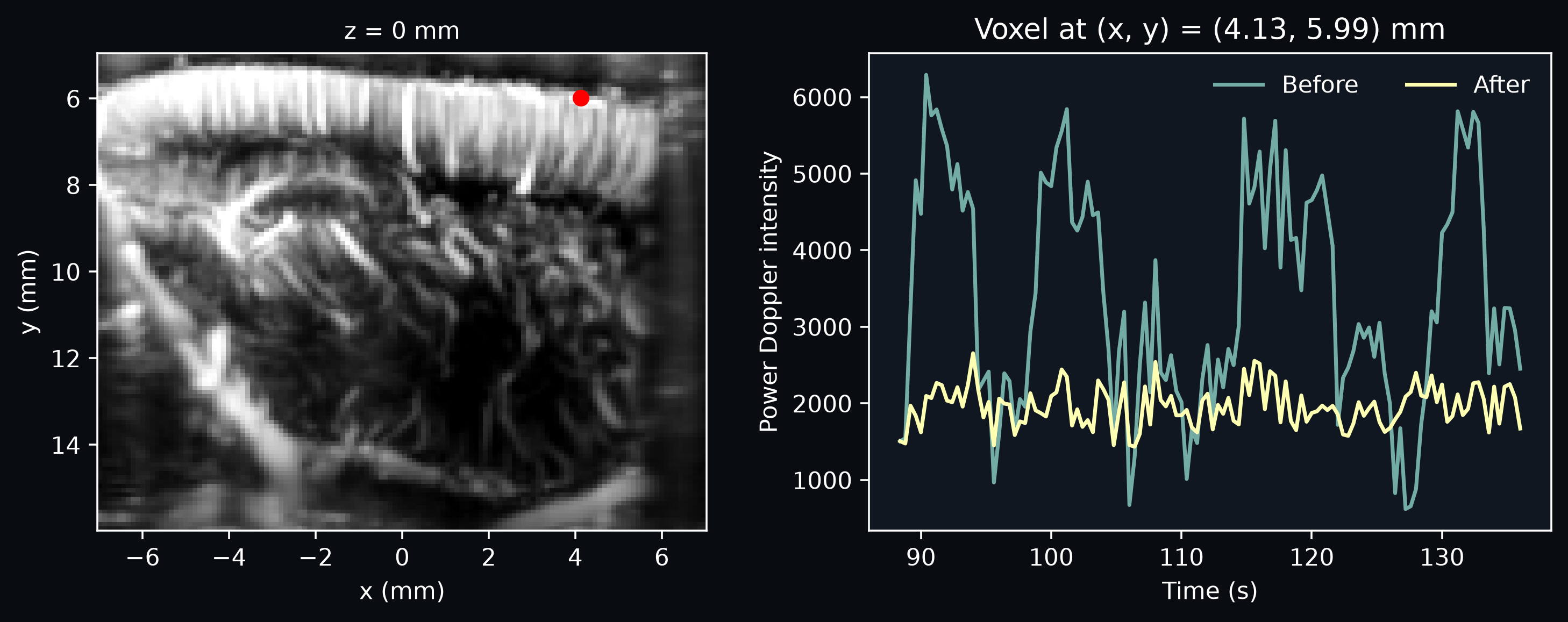
To highlight the effect of the volumewise registration, we pick the voxel with the largest temporal standard deviation in the unregistered recording. In practice that usually lands on a large vessel or near the borders of the brain, where brain motion can induce high intensity changes.

std_map = data.std("time")
highest_std_voxel = std_map.isel(std_map.argmax(dim=["x", "y", "z"]))

voxel_before = data.sel(highest_std_voxel.coords)
voxel_after = registered.sel(highest_std_voxel.coords)

x_value = highest_std_voxel.x.values
y_value = highest_std_voxel.y.values
units = highest_std_voxel.x.units
xy_position = f"(x, y) = ({x_value:.2f}, {y_value:.2f}) {units}"

fig, axs = plt.subplots(1, 2, figsize=(9, 3.5), constrained_layout=True)
fig.patch.set_facecolor(bg_color)

plotter = (
    data.mean("time")
    .fusi.scale.db()
    .fusi.plot.volume(axes=axs[0], bg_color=bg_color, show_colorbar=False)
)

# Explicitly show the high std voxel on the brain plot.
axs[0].scatter(highest_std_voxel.x, highest_std_voxel.y, color="r")

axs[1].plot(voxel_before["time"], voxel_before, label="Before", lw=1.6, alpha=0.8)
axs[1].plot(voxel_after["time"], voxel_after, label="After", lw=1.6)
axs[1].set_xlabel("Time (s)")
axs[1].set_ylabel("Power Doppler intensity")
axs[1].set_title(f"Voxel at {xy_position}")
_ = axs[1].legend(frameon=False, ncols=2)

Check the alignment over time¶

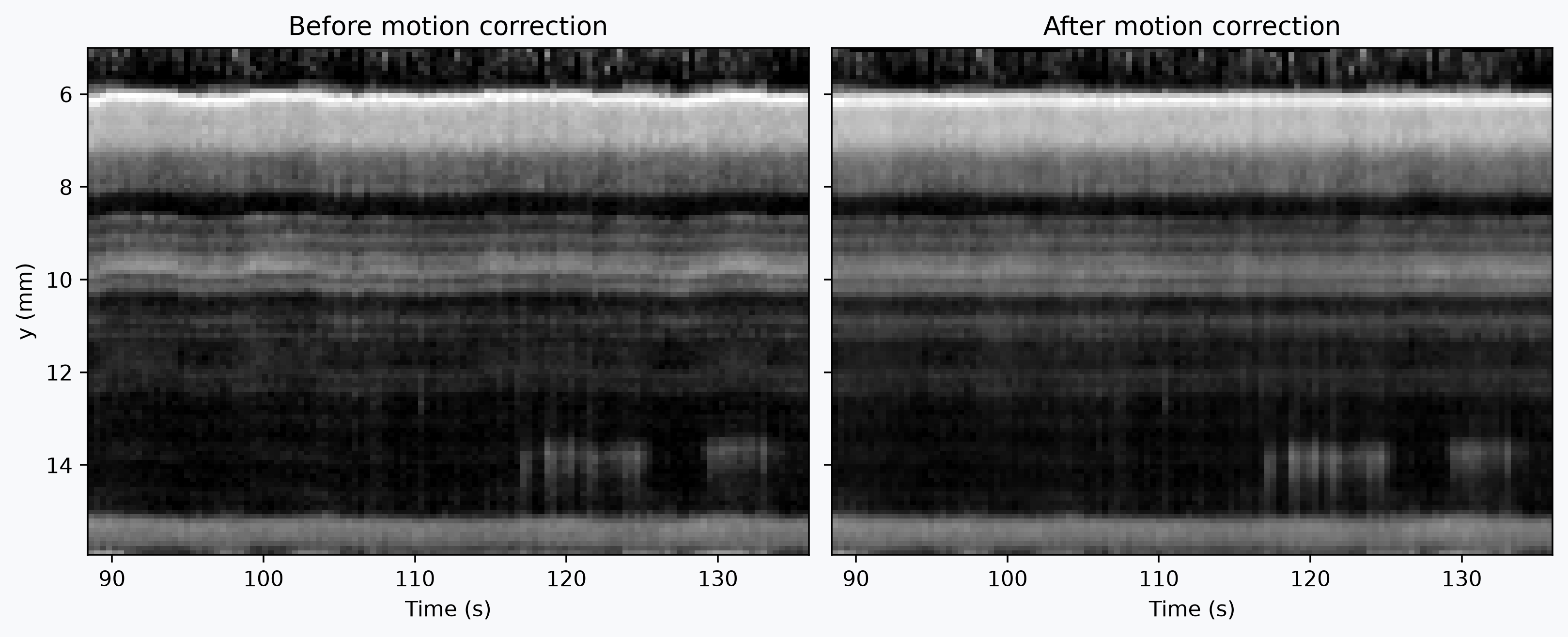
A compact way to inspect the correction inside the notebook is to follow one column across time. Motion appears as slanted or wobbling vessel traces in this y × time raster, while a good correction makes those traces more horizontal and stable (note that this will only clearly capture translation motion in the y axis).

raster_before = data.fusi.scale.db().sel(z=0, x=x_value)
raster_after = registered.fusi.scale.db().sel(z=0, x=x_value)

fig, axes = plt.subplots(1, 2, figsize=(10, 4), constrained_layout=True, sharey=True)
fig.patch.set_facecolor(bg_color)

vmin = float(np.nanpercentile(raster_before, 2))
vmax = float(np.nanpercentile(raster_before, 99.8))

for ax, raster, title in [
    (axes[0], raster_before, "Before motion correction"),
    (axes[1], raster_after, "After motion correction"),
]:
    ax.imshow(
        raster.T,
        aspect="auto",
        origin="upper",
        cmap="gray",
        vmin=vmin,
        vmax=vmax,
        extent=[
            float(raster["time"].values[0]),
            float(raster["time"].values[-1]),
            float(raster["y"].values[-1]),
            float(raster["y"].values[0]),
        ],
    )
    ax.set_title(title)
    ax.set_xlabel("Time (s)")

_ = axes[0].set_ylabel("y (mm)")

For a full visual check of the corrected movie, open the result in napari with plot_napari or inspect it in the ConfUSIus plugin. We intentionally do not embed a full before/after GIF here because it would make the rendered notebook unnecessarily heavy. For a full preprocessing workflow, you would usually run the same correction on the complete recording before downstream QC, decomposition, or connectivity analysis.

Total running time: 41.6 s

Launch in Binder Download .py Download .ipynb

Power, J. D., Barnes, K. A., Snyder, A. Z., Schlaggar, B. L. & Petersen, S. E. Spurious but systematic correlations in functional connectivity MRI networks arise from subject motion. Neuroimage 59, 2142-2154 ↩↩