Register a recording to an Allen fUSI template¶

This example shows the full workflow for aligning a single-slice fUSI recording to one of ConfUSIus's Allen-space fUSI templates: fetch the recording and the template, initialize and refine the registration, inspect diagnostic overlays, resample the Allen Mouse Brain Atlas onto the recording's native grid, and save the aligned atlas for reuse.

We use an awake freely-running acquisition from subject CR022, session 20201007, in the Nunez-Elizalde 2022 dataset, and the Pepe, Mariani 2026 fUSI template, which carries the affine transform required to bring it into Allen Common Coordinate Framework (CCF) space.

Fetch the recording and the template¶

The recording is a single coronal slice imaged for approximately 4 minutes at 3.33 Hz. Registration works on a static anatomical image, so we use the temporal mean, converted to decibels for a more stable dynamic range.

from pathlib import Path

import matplotlib as mpl
import matplotlib.pyplot as plt
import numpy as np
import xarray as xr

import confusius as cf

# Adapt background color to the current Matplotlib style.
bg_color = mpl.colors.to_hex(mpl.rcParams["figure.facecolor"])

xr.set_options(display_expand_data=False)

# The ConfUSIus datasets directory is a convenient place to cache the resampled atlas.
CONFUSIUS_DATA_DIR = cf.datasets.get_datasets_dir()

template = cf.datasets.fetch_template_pepe_mariani_2026().compute()

bids_root = cf.datasets.fetch_nunez_elizalde_2022(
    subjects="CR022", sessions="20201007", tasks="spontaneous", acqs="slice02"
)

If you use this template in your work, please cite the following source:

Pepe, C., Mariani, J.-C., Urosevic, M., Gini, S., Stuefer, A., Ricci, F., Galbusera, A., Iurilli, G., & Gozzi, A. 
(2026). Structural and dynamic embedding of the mouse functional connectome revealed by functional ultrasound 
imaging (fUSI). bioRxiv. https://doi.org/10.64898/2026.02.05.704055

If you use this dataset in your work, please cite the following source:

Nunez-Elizalde, A. O., Krumin, M., Reddy, C. B., Montaldo, G., Urban, A., Harris, K. D., & Carandini, M. (2022). 
Neural correlates of blood flow measured by ultrasound. Neuron, 110(10), 1631–1640.e4. 
https://doi.org/10.1016/j.neuron.2022.02.012

data_path = (
    Path(bids_root)
    / "sub-CR022"
    / "ses-20201007"
    / "fusi"
    / "sub-CR022_ses-20201007_task-spontaneous_acq-slice02_pwd.nii.gz"
)
moving = cf.load(data_path).mean(dim="time").fusi.scale.db().compute()

moving

xarray.DataArray

'sub-CR022_ses-20201007_task-spontaneous_acq-slice02_pwd'

z: 1
y: 125
x: 80

-18.69 -18.57 -18.5 -18.46 -18.38 ... -13.37 -13.36 -13.33 -13.28

array([[[-18.687603 , -18.568825 , -18.500853 , ..., -17.956799 ,
         -17.938179 , -17.963793 ],
        [-18.534925 , -18.445103 , -18.356045 , ..., -17.885395 ,
         -17.88491  , -17.891798 ],
        [-18.489155 , -18.406622 , -18.328014 , ..., -17.79321  ,
         -17.804344 , -17.829521 ],
        ...,
        [-12.314958 , -13.393738 , -13.82475  , ..., -13.536392 ,
         -13.5213375, -13.627226 ],
        [-12.319061 , -13.352966 , -13.748854 , ..., -13.4567585,
         -13.385921 , -13.444569 ],
        [-12.375978 , -13.218855 , -13.602357 , ..., -13.363947 ,
         -13.333372 , -13.279113 ]]], shape=(1, 125, 80), dtype=float32)

Coordinates: (3)

z
(z)
float64
0.4
units :
mm
voxdim :
0.4000000059604645
```
array([0.4])
```

y

(y)

float64

2.996 3.044 3.092 ... 8.939 8.988

units :: mm
voxdim :: 0.04831999912858009

array([2.99584, 3.04416, 3.09248, 3.1408 , 3.18912, 3.23744, 3.28576, 3.33408,
       3.3824 , 3.43072, 3.47904, 3.52736, 3.57568, 3.624  , 3.67232, 3.72064,
       3.76896, 3.81728, 3.8656 , 3.91392, 3.96224, 4.01056, 4.05888, 4.1072 ,
       4.15552, 4.20384, 4.25216, 4.30048, 4.3488 , 4.39712, 4.44544, 4.49376,
       4.54208, 4.5904 , 4.63872, 4.68704, 4.73536, 4.78368, 4.832  , 4.88032,
       4.92864, 4.97696, 5.02528, 5.0736 , 5.12192, 5.17024, 5.21856, 5.26688,
       5.3152 , 5.36352, 5.41184, 5.46016, 5.50848, 5.5568 , 5.60512, 5.65344,
       5.70176, 5.75008, 5.7984 , 5.84672, 5.89504, 5.94336, 5.99168, 6.04   ,
       6.08832, 6.13664, 6.18496, 6.23328, 6.2816 , 6.32992, 6.37824, 6.42656,
       6.47488, 6.5232 , 6.57152, 6.61984, 6.66816, 6.71648, 6.7648 , 6.81312,
       6.86144, 6.90976, 6.95808, 7.0064 , 7.05472, 7.10304, 7.15136, 7.19968,
       7.248  , 7.29632, 7.34464, 7.39296, 7.44128, 7.4896 , 7.53792, 7.58624,
       7.63456, 7.68288, 7.7312 , 7.77952, 7.82784, 7.87616, 7.92448, 7.9728 ,
       8.02112, 8.06944, 8.11776, 8.16608, 8.2144 , 8.26272, 8.31104, 8.35936,
       8.40768, 8.456  , 8.50432, 8.55264, 8.60096, 8.64928, 8.6976 , 8.74592,
       8.79424, 8.84256, 8.89088, 8.9392 , 8.98752])

x

(x)

float64

-3.95 -3.85 -3.75 ... 3.85 3.95

units :: mm
voxdim :: 0.10000000149011612

array([-3.95, -3.85, -3.75, -3.65, -3.55, -3.45, -3.35, -3.25, -3.15, -3.05,
       -2.95, -2.85, -2.75, -2.65, -2.55, -2.45, -2.35, -2.25, -2.15, -2.05,
       -1.95, -1.85, -1.75, -1.65, -1.55, -1.45, -1.35, -1.25, -1.15, -1.05,
       -0.95, -0.85, -0.75, -0.65, -0.55, -0.45, -0.35, -0.25, -0.15, -0.05,
        0.05,  0.15,  0.25,  0.35,  0.45,  0.55,  0.65,  0.75,  0.85,  0.95,
        1.05,  1.15,  1.25,  1.35,  1.45,  1.55,  1.65,  1.75,  1.85,  1.95,
        2.05,  2.15,  2.25,  2.35,  2.45,  2.55,  2.65,  2.75,  2.85,  2.95,
        3.05,  3.15,  3.25,  3.35,  3.45,  3.55,  3.65,  3.75,  3.85,  3.95])

Attributes: (27)
qform_code :
1
manufacturer :
Verasonics
manufacturers_model_name :
Vantage 128
software_version :
Alan Urban Technology & Consulting (AUTC)
probe_manufacturer :
Vermon
probe_type :
linear
probe_model :
L22-XTech
probe_central_frequency :
15000000.0
probe_number_of_elements :
128
probe_pitch :
0.1
probe_focal_width :
0.4
probe_focal_depth :
8.0
power_doppler_integration_duration :
0.3
power_doppler_integration_stride :
0.3
clutter_filter_window_duration :
0.4
clutter_filter_window_stride :
0.3
clutter_filters :
['highpass:15Hz', 'svd:remove_first_15_components']
task_name :
spontaneous
task_description :
Spontaneous activity without explicit visual stimulation.
depth :
[0.0, 5.991680000000001]
transmit_frequency :
15625000.0
compound_sampling_frequency :
500.0
plane_wave_angles :
[-10.0, -7.9, -5.8, -3.6999999999999993, -1.5999999999999996, 0.5000000000000018, 2.6000000000000014, 4.700000000000002, 6.8000000000000025, 8.900000000000002]
probe_voltage :
25.0
affines :
{'physical_to_qform': array([[1., 0., 0., 0.], [0., 1., 0., 0.], [0., 0., 1., 0.], [0., 0., 0., 1.]])}
units :
dB
scaling :
10*log10(x/max)

Register the recording to the template¶

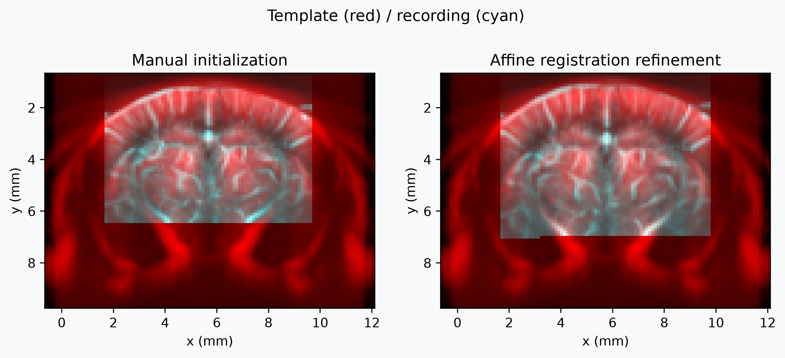
The template is a 3D volume but the recording is a single slice. We can still register the recording to the template, but we need to initialize the registration with a rough guess of where the recording sits in the template, otherwise the registration algorithm may not converge to the right slice. To initialize the registration, we use an affine transform obtained using napari's manual transform tool by placing the recording at an approximate location on the template. The transform is not perfect (notice the slight misalignment toward the bottom of the field of view), but it is close enough to allow the registration algorithm to converge to a good solution.

register_volume expects a transform mapping fixed (template) physical coordinates to moving (recording) physical coordinates, so we invert the napari affine—which instead describes how to place the recording into the template's coordinate system—before using it as initialization.

# Copied and pasted transform after manual transformation in napari.
napari_affine = np.array(
    [
        [1.0, 0.0, 0.0, 5.594638656430411],
        [0.0, 1.0, 0.0, -2.50293925701927],
        [0.0, 0.0, 1.0, 5.6650243788545875],
        [0.0, 0.0, 0.0, 1.0],
    ]
)
initialization = np.linalg.inv(napari_affine)

# Crop the template to a thin band around the recording's expected location to improve
# registration speed and visualization.
target_z = napari_affine[0, 3] + float(moving.z.values[0])
fixed = template.sel(z=slice(target_z - 1.0, target_z + 1.0)).fusi.scale.db()

initialized = cf.registration.resample_like(moving, fixed, initialization)
_ = cf.plotting.plot_composite(
    fixed,
    initialized,
    slice_coords=[target_z],
    normalize_strategy="per_slice",
    bg_color=bg_color,
)

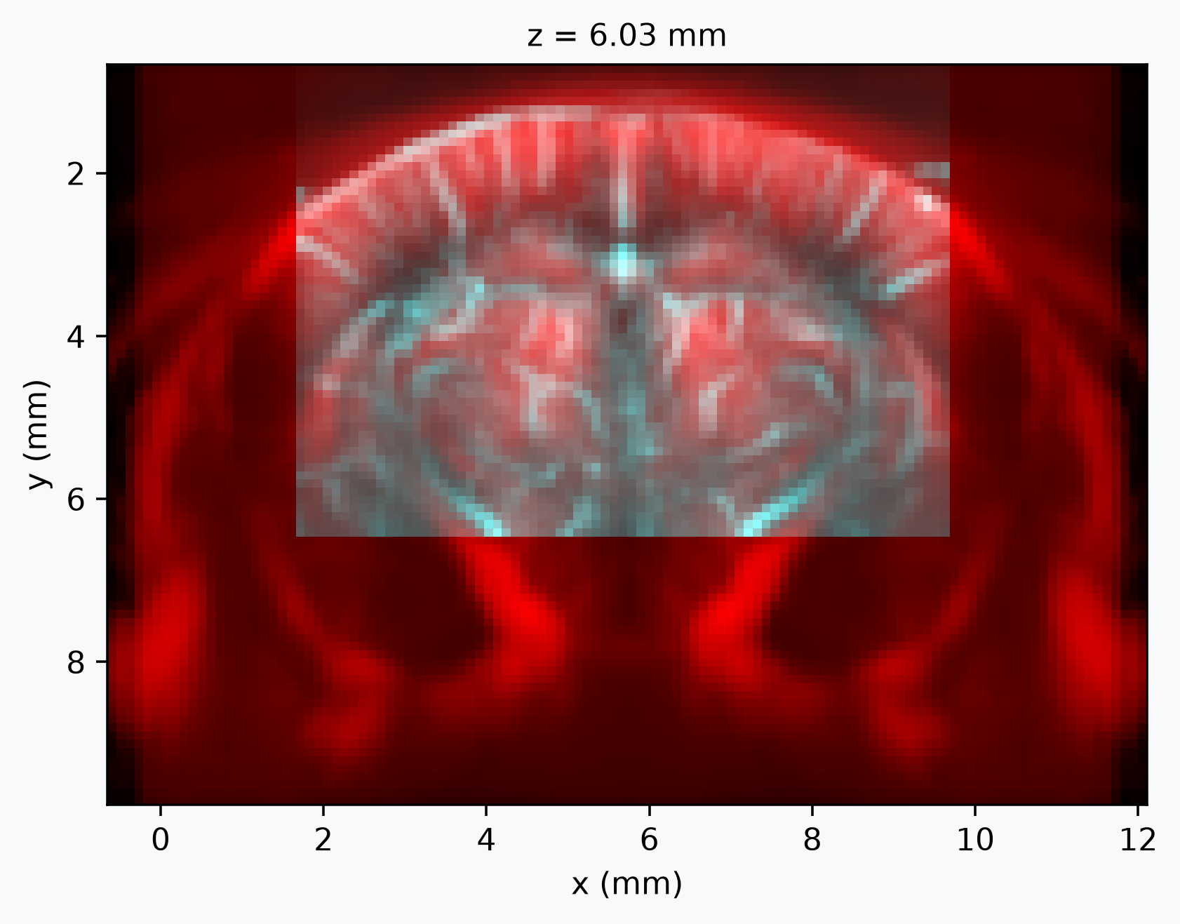
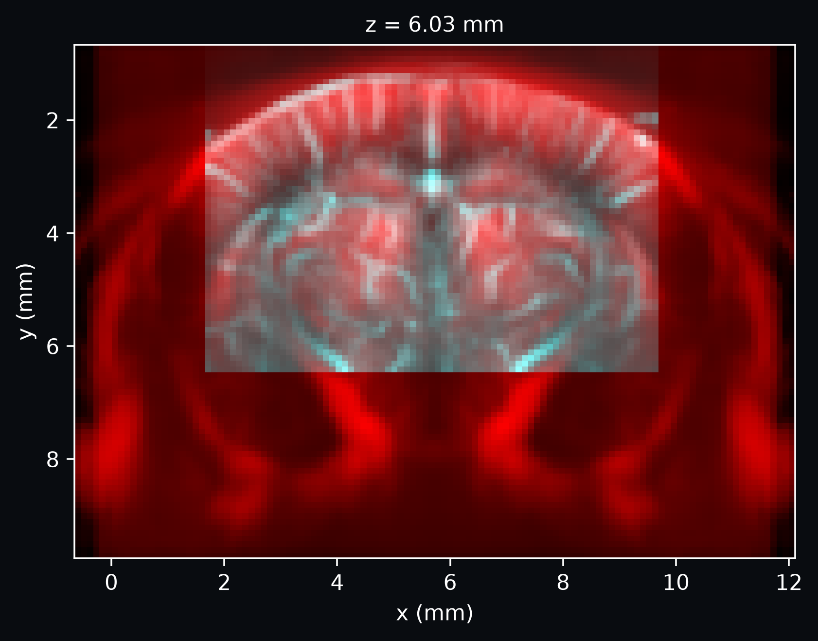
We use an affine transform: on top of the rotation and translation a rigid transform would allow, it also captures small scale and shear differences between the recording and the template.

registered, affine, _ = cf.registration.register_volume(
    moving=moving,
    fixed=fixed,
    transform_type="affine",
    metric="correlation",
    convergence_window_size=50,
    number_of_iterations=500,
    learning_rate=1,
    initialization=initialization,
    show_progress=True,
)

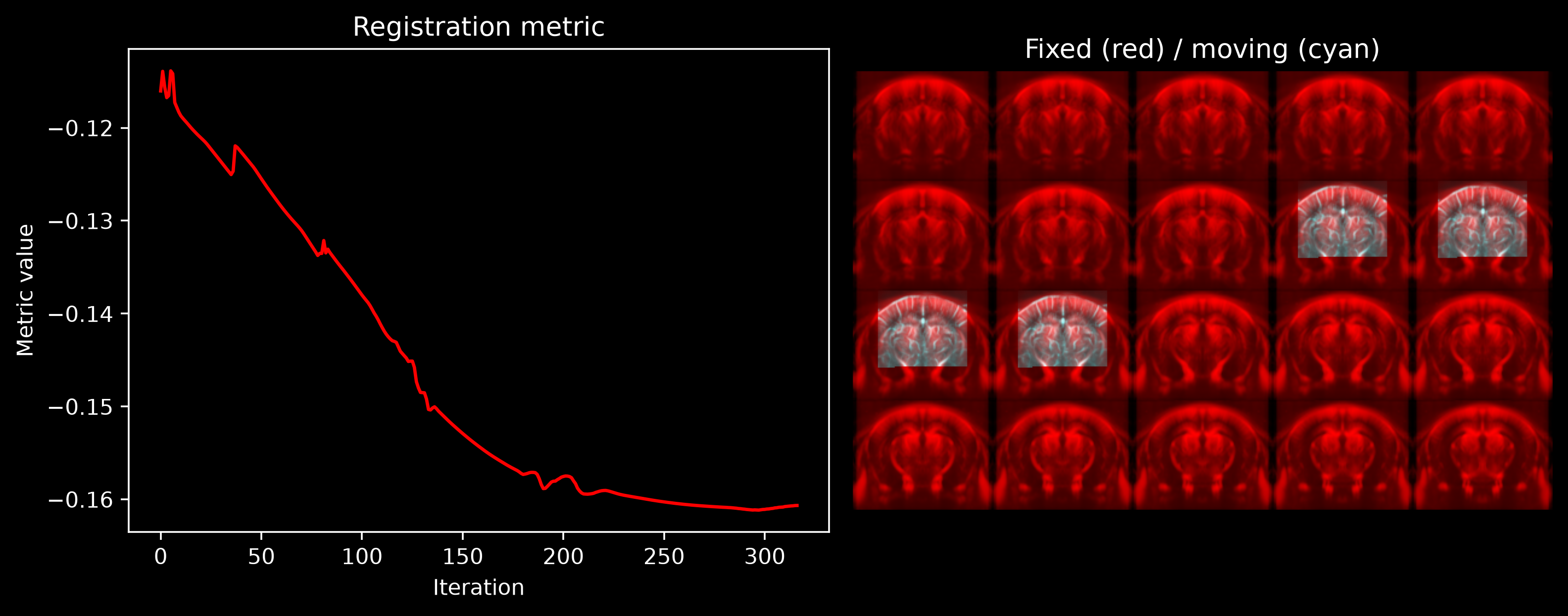
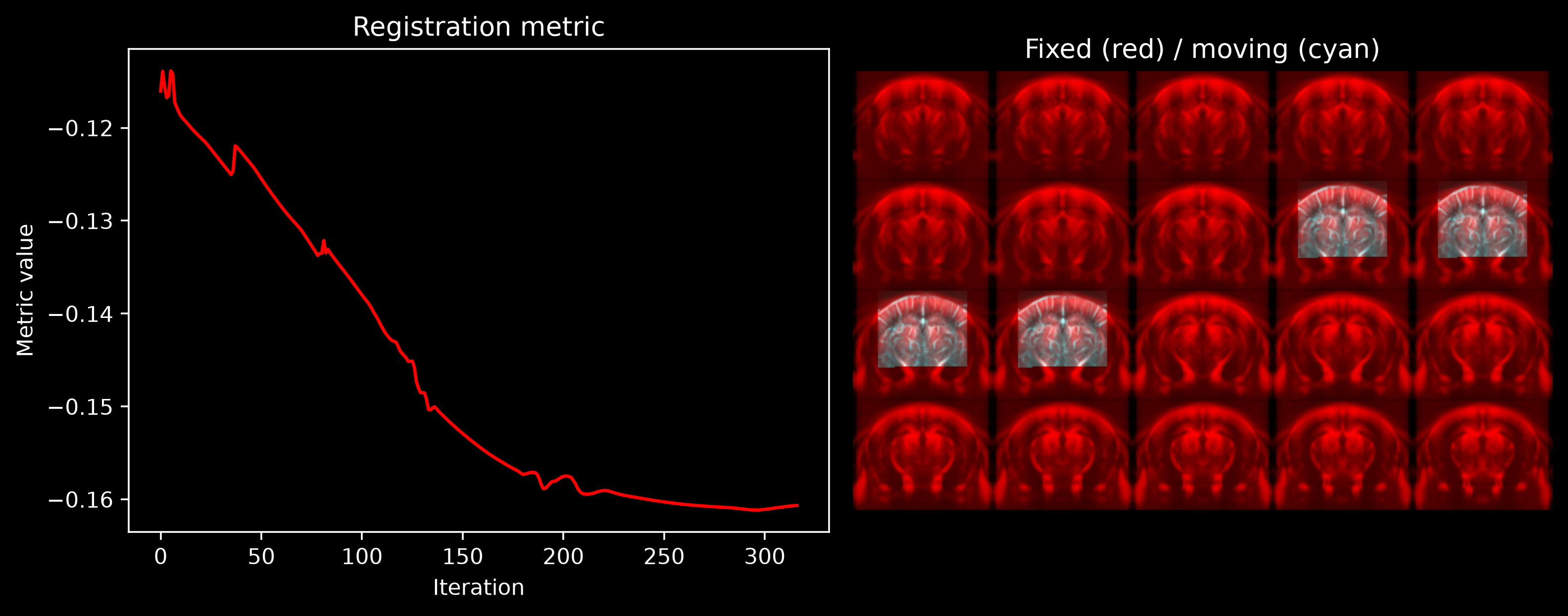
The initialization was already close, so the refinement is small. Comparing the overlay before and after registration, alignment is slightly better after the affine refinement, most noticeably around the anterior choroidal arteries in the bottom part of the field of view.

fig, axes = plt.subplots(1, 2, figsize=(10, 4))
fig.patch.set_facecolor(bg_color)
for ax, moving_view, title in [
    (axes[0], initialized, "Manual initialization"),
    (axes[1], registered, "Affine registration refinement"),
]:
    cf.plotting.plot_composite(
        fixed,
        moving_view,
        axes=ax,
        slice_coords=[target_z],
        normalize_strategy="per_slice",
        bg_color=bg_color,
    )
    ax.set_title(title)

_ = fig.suptitle("Template (red) / recording (cyan)")

Resample the Allen atlas onto the recording's native grid¶

The template is not itself expressed in Allen space, but it carries the affine transform to get there in template.attrs["affines"]["physical_to_sform"]. Composing it with the inverse of the estimated registration affine gives a single transform from the recording's native coordinates directly to Allen atlas coordinates.

resample_like then brings the atlas's reference volume, annotations, and hemisphere map onto the recording's grid in one call.

physical_to_sform = template.attrs["affines"]["physical_to_sform"]
subject_to_atlas = physical_to_sform @ np.linalg.inv(affine)

atlas = cf.datasets.fetch_brainglobe_atlas("allen_mouse_100um", check_latest=False)
resampled_atlas = atlas.atlas.resample_like(moving, subject_to_atlas)

Save and reload the resampled atlas¶

Registration and atlas resampling are expensive, so for downstream analyses of the same recording it is worth caching the aligned atlas once and reloading it later. save_atlas writes the arrays together with the structure hierarchy and meshes, so the reloaded atlas is immediately usable for masks, meshes, and plotting.

store_path = f"{CONFUSIUS_DATA_DIR}/resampled_allen_mouse_100um.zarr"
cf.io.save_atlas(resampled_atlas, store_path, mode="w")
del resampled_atlas

resampled_atlas = cf.io.load_atlas(store_path)

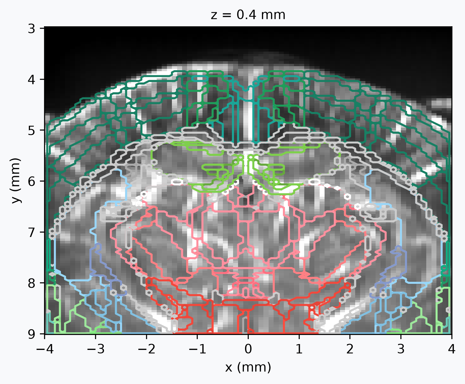
plotter = cf.plotting.plot_volume(
    moving, slice_mode="z", cmap="gray", show_colorbar=False, bg_color=bg_color
)
_ = plotter.add_contours(resampled_atlas.annotation)

Total running time: 217.9 s

Launch in Binder Download .py Download .ipynb