Lagged first-level GLM analysis of fUSI data with a continuous regressor¶

This example reproduces the lagged-GLM analysis reported by Cybis Pereira et al. 2026, which uses functional ultrasound imaging of a freely moving rat exploring an open field with its body position tracked from video. Unlike the block-design task in the First-level GLM analysis of fUSI data example, the regressor of interest is a continuous variable measured throughout the recording, the animal's locomotion speed, and we ask at every voxel how much of the power Doppler time course tracks it at different lags.

Rather than convolving the speed regressor with a hemodynamic response function, the analysis shifts it across a range of temporal lags and fits one model per lag, much like a voxel-wise cross-correlation between speed and the vascular signal. The notebook goes through:

Fetch and load one open-field recording and its motion track.
Build an animal speed regressor from the animal's pose estimation.
Encode speed as a per-volume parametric modulator and extract CompCor noise regressors.
Fit a FirstLevelModel at a range of temporal lags between speed and signal.
Threshold the resulting maps and visualize the response at each lag.

Fetch the recording¶

fetch_cybis_pereira_2026 downloads the fUSI-BIDS dataset. We take subject rat75, session 20220524, acquisition slice32 of the openfield task, which gives one power Doppler recording together with its motion track.

from pathlib import Path

import matplotlib as mpl
import matplotlib.pyplot as plt
import numpy as np
import pandas as pd
import xarray as xr

import confusius as cf

# Adapt background color to the current Matplotlib style.
bg_color = mpl.colors.to_hex(mpl.rcParams["figure.facecolor"])
is_dark_theme = sum(mpl.colors.to_rgb(bg_color)) / 3 < 0.5

# Keep notebook output compact for large DataArray displays. The coordinates section is
# left expanded on purpose; `display_expand_data` alone does not cover the attributes.
xr.set_options(display_expand_data=False, display_expand_attrs=False)

subject = "rat75"
session = "20220524"
acq = "slice32"

bids_root = cf.datasets.fetch_cybis_pereira_2026(
    datasets="rawdata",
    subjects=subject,
    sessions=session,
    acqs=acq,
)

pwd_path = (
    Path(bids_root)
    / f"sub-{subject}"
    / f"ses-{session}"
    / "fusi"
    / f"sub-{subject}_ses-{session}_task-openfield_acq-{acq}_pwd.nii.gz"
)

motion_path = (
    Path(bids_root)
    / f"sub-{subject}"
    / f"ses-{session}"
    / "motion"
    / f"sub-{subject}_ses-{session}_task-openfield_tracksys-DLC_acq-{acq}_motion.tsv"
)

If you use this dataset in your work, please cite the following source:

Cybis Pereira, F., Castedo, S. H., Meur-Diebolt, S. L., Ialy-Radio, N., Bhattacharya, S., Ferrier, J., Osmanski, B.
F., Cocco, S., Monasson, R., Pezet, S., & Tanter, M. (2026). A vascular code for speed in the spatial navigation 
system. Cell Reports, 45(1). https://doi.org/10.1016/j.celrep.2025.116791

Load the recording¶

cf.load reads the power Doppler NIfTI into an xarray.DataArray. We call .compute() to pull it fully into memory, since it is reused across many model fits below.

data = cf.load(pwd_path).compute()
data

Correct for motion¶

The rat moves freely, so a real analysis should first correct volume-to-volume brain motion. We skip it here to keep the example fast to build, at the cost of a little statistical robustness in the maps below.

Recommended in a real analysis

Register every volume to a reference frame with register_volumewise before building the regressors, then continue with the corrected data. Removing motion-driven variance sharpens the speed maps and their statistics. See the Motion correction of a single recording example for the full workflow and diagnostics.

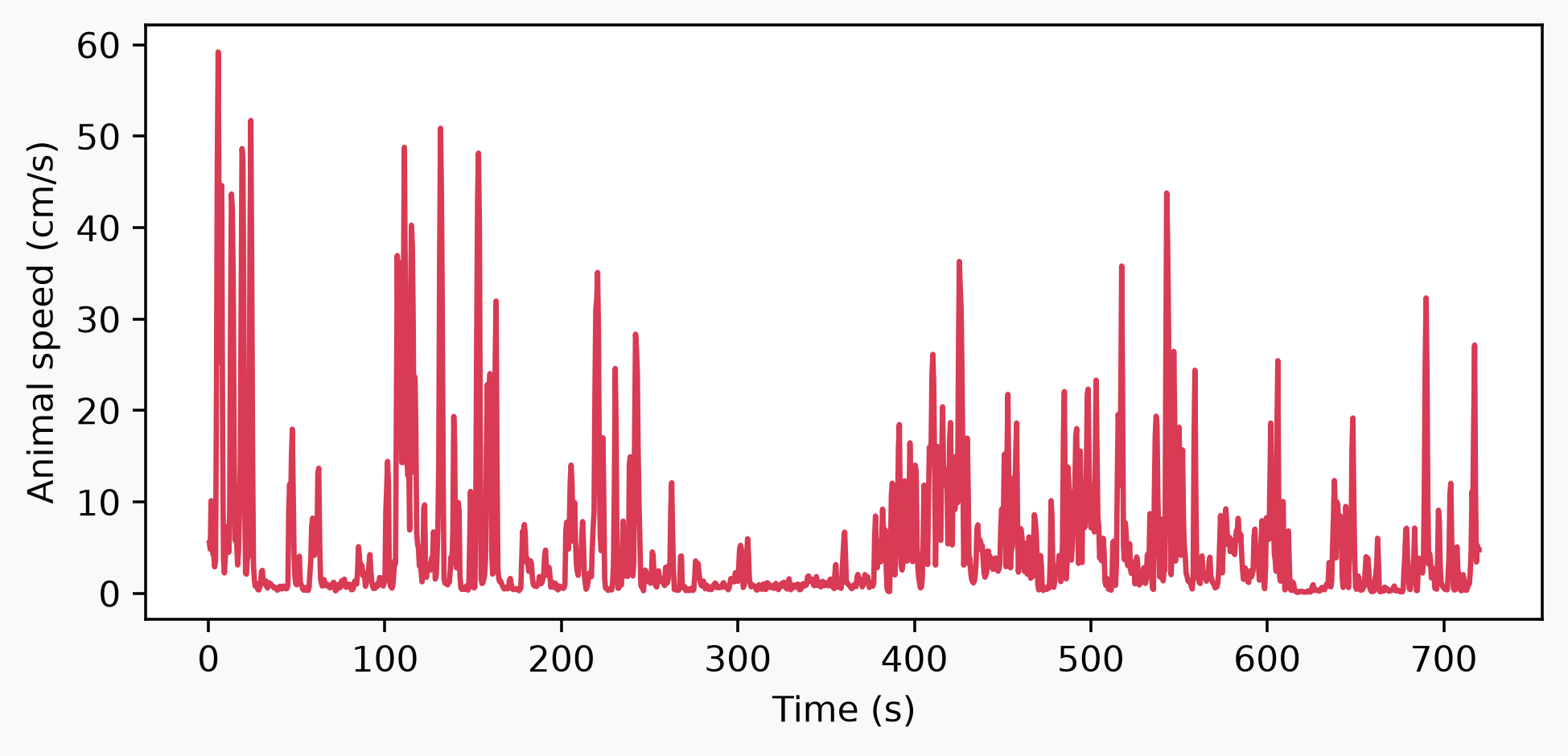
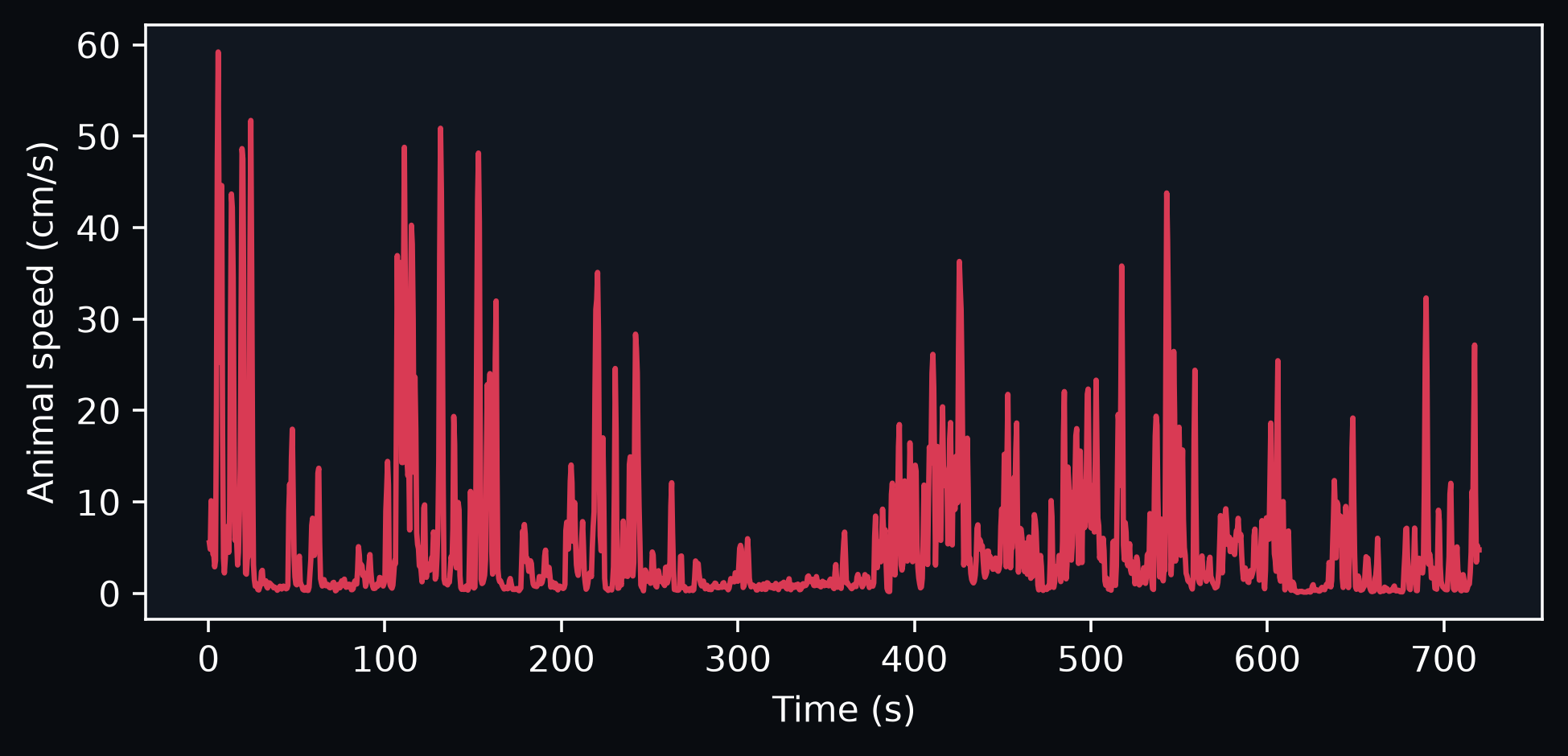
data = cf.registration.register_volumewise(data, learning_rate=1)

Build the animal speed regressor from the pose estimation¶

The motion .tsv holds the body position (body_x, body_y) tracked with DeepLabCut at 50 fps. We take the frame-to-frame Euclidean displacement, scale it by the frame rate to obtain speed, smooth it with a 1 s centered rolling mean, and resample it onto the fUSI volume times.

fps = 50
motion_df = pd.read_csv(motion_path, sep="\t")
squared_diff = motion_df.diff() ** 2
speed_df = fps * (squared_diff["body_x"] + squared_diff["body_y"]) ** 0.5
speed_df[0] = 0
speed = (
    xr.DataArray(
        speed_df,
        dims=["time"],
        coords={"time": 1 / fps * np.arange(len(speed_df))},
        name="speed",
    )
    .rolling(time=fps, min_periods=1, center=True)
    .mean()
)
speed = speed.interp(time=data.time, method="linear").ffill("time")

fig, ax = plt.subplots(figsize=(7, 3), facecolor=bg_color)
ax.plot(speed.time, speed, color="#d93a54")
ax.set_xlabel("Time (s)")
_ = ax.set_ylabel("Animal speed (cm/s)")

Encode speed as a parametric modulator¶

We build an events table with one entry per fUSI volume, each carrying the speed at that volume as its modulation, which turns speed into a single continuous regressor.

events = pd.DataFrame(
    {
        "onset": data.time,
        "duration": [data.time.volume_acquisition_duration] * len(data),
        "modulation": speed,
        "trial_type": ["speed"] * len(data),
    }
)

Model physiological noise with CompCor¶

compute_compcor_confounds extracts the three leading principal components of the highest-variance voxels (the top 5%) to add as nuisance regressors (temporal CompCor).

confounds = cf.signal.compute_compcor_confounds(
    data,
    variance_threshold=0.05,
    n_components=3,
)

Build the model and design matrix¶

We instantiate the FirstLevelModel with a light 0.3 mm Gaussian spatial smoothing (the default AR(1) noise model handles temporal autocorrelation) and build the design matrix with make_first_level_design_matrix: the speed regressor, the CompCor confounds, a "cosine" drift basis that high-pass filters drifts below 0.01 Hz, and a constant.

glm = cf.glm.FirstLevelModel(smoothing_fwhm=0.3)
design_matrix = cf.glm.make_first_level_design_matrix(
    data.time.values,
    events=events,
    drift_model="cosine",
    low_cutoff=0.01,
    confounds=confounds,
)

Fit the GLM across temporal lags¶

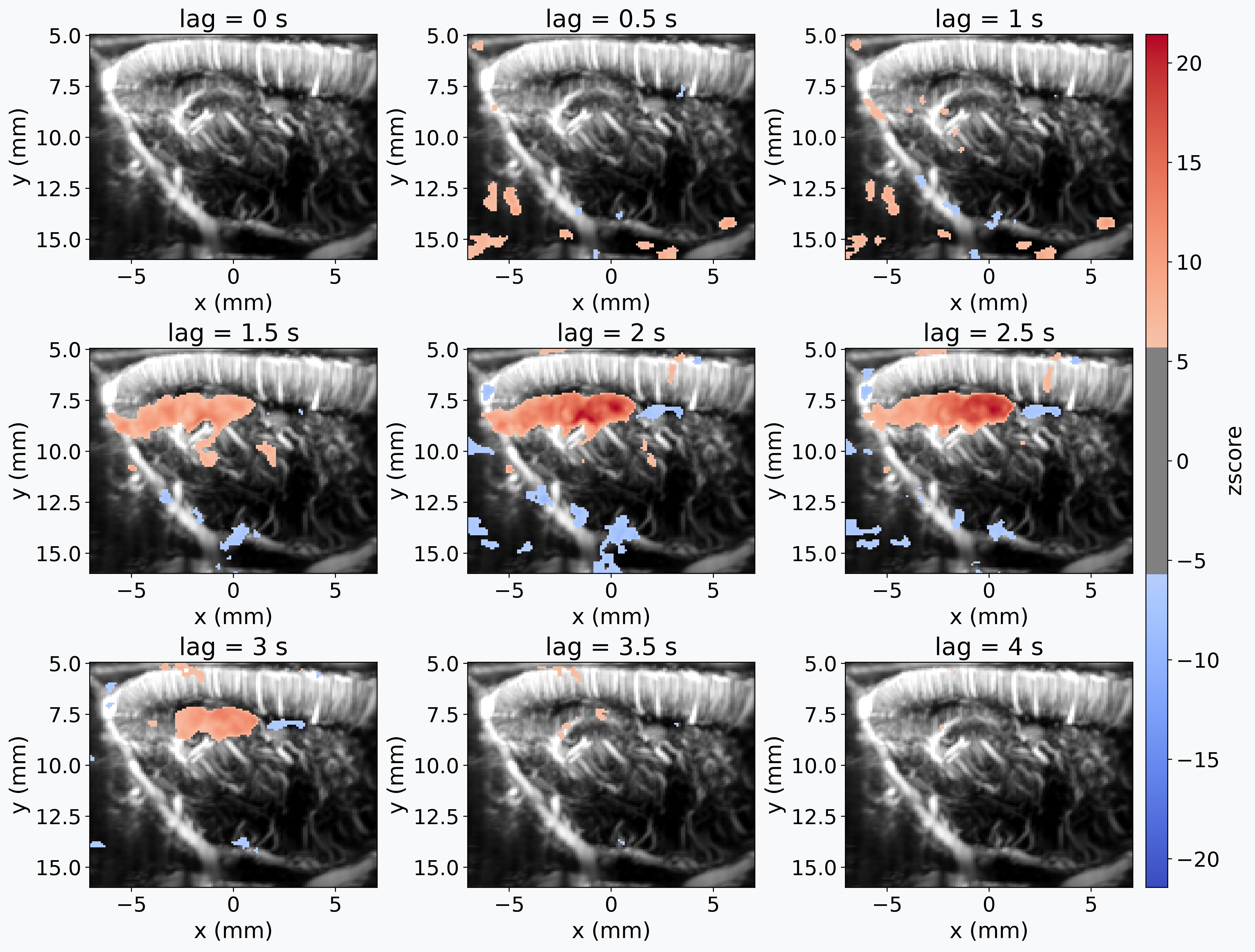
The vascular response follows a change in speed with a delay. Instead of fixing that delay with an HRF, we sweep it: for each temporal lag we shift only the speed regressor, leaving the confounds, drift, and data window fixed. We fit the model, and compute the "speed" contrast. This yields one z-map per lag, like a cross-correlation between speed and the signal of each voxel. Holding the window fixed across lags keeps the maps comparable, and a positive lag means the signal responds after the change in speed. run_lagged_glm returns the per-lag maps, which we stack along a lag dimension whose coordinate is the delay in seconds (one volume per lag). The original study sweeps a wider window (about -2 to 10 s); here we use a short positive range to keep the example quick.

def run_lagged_glm(
    data: xr.DataArray,
    glm: cf.glm.FirstLevelModel,
    design_matrix: pd.DataFrame,
    lags: range,
) -> list[xr.DataArray]:
    """Fit the GLM at a range of lags, shifting only the speed regressor."""
    max_lag = max(lags)
    n = len(design_matrix)

    # Fixed data window and time-locked nuisance regressors, shared by every lag.
    data_window = data[max_lag:]
    fixed_design = design_matrix.iloc[max_lag:]

    z_scores = []
    for lag in lags:
        design = fixed_design.copy()
        # Shift only the regressor of interest: speed at volume t - lag predicts the
        # signal at volume t.
        design["speed"] = design_matrix["speed"].iloc[max_lag - lag : n - lag].values
        glm.fit([data_window], design_matrices=[design])
        z_scores.append(glm.compute_contrast("speed"))

    return z_scores


lags = range(9)
z_scores = run_lagged_glm(data, glm, design_matrix, lags=lags)
z_score = xr.concat(z_scores, dim="lag").assign_coords(
    lag=data.fusi.spacing["time"] * np.asarray(lags)
)
z_score.lag.attrs["units"] = data.time.units

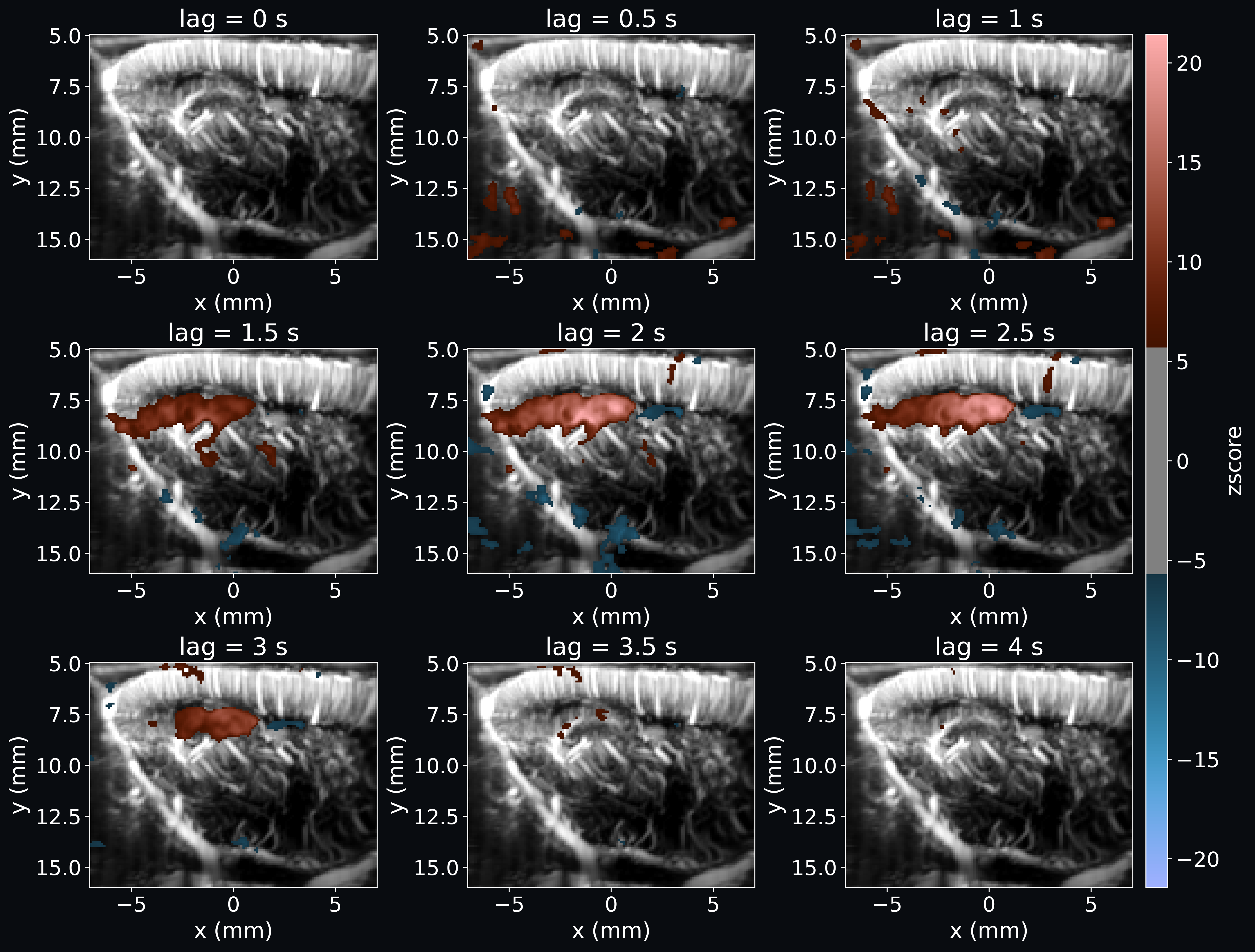
Threshold and display the maps¶

apply_statistical_threshold applies a Bonferroni correction at alpha=0.001 followed by a 30-voxel cluster-extent threshold, zeroing the voxels that do not survive. We plot the thresholded z-map at each lag over the mean power Doppler image (in dB).

thresholded_zscore, threshold = cf.stats.apply_statistical_threshold(
    z_score,
    alpha=0.001,
    method="bonferroni",
    cluster_threshold=30,
)

cmap = "berlin" if is_dark_theme else None
_ = thresholded_zscore.fusi.plot.stat_map(
    bg_volume=data.mean("time").fusi.scale.db().expand_dims(lag=z_score.lag),
    slice_mode="lag",
    nrows=3,
    cmap=cmap,
    threshold=threshold,
    bg_color=bg_color,
    fontsize=20,
)

Total running time: 28.5 s

Launch in Binder Download .py Download .ipynb