First-level GLM analysis of fUSI data
The General Linear Model (GLM) is the workhorse of task-based neuroimaging analysis. It treats every voxel independently and asks a simple question: how much of this voxel's time course can be explained by the experimental paradigm, once we account for nuisance signals such as slow drifts and physiological noise? Fitting that model voxel-by-voxel turns a fUSI recording into a statistical map that highlights where the brain responded to the stimulus.
In this example we run a complete first-level (single-subject) GLM on stimulus-evoked fUSI data from the Khallaf et al. 2026 dataset—functional ultrasound imaging of a naked mole-rat exposed to repeated olfactory stimulation. The notebook will go through the following steps:
- Fetch and load the five fUSI recordings.
- Register the recording to a reference template aligned with an anatomical atlas, so we can define masks and draw region boundaries in a common space.
- Choose a fUSI-specific HRF and extract CompCor noise regressors from a non-task region.
- Fit a
FirstLevelModelacross all runs and compute a contrast for the stimulation condition. - Threshold the resulting map for statistical significance and visualize it.
Download size
Running this notebook fetches the five recordings for subject 5622, session
IPM (about 200 MB each, ~1 GB in total) into the ConfUSIus dataset cache.
Fetch the olfactory-stimulation recordings
Using fetch_khallaf_2026,
we take subject 5622, session IPM, and the resampled reconstruction (the runs
already aligned to a common within-session space), which yields five task runs.
import warnings
from functools import partial
from pathlib import Path

import matplotlib as mpl
import matplotlib.pyplot as plt
import numpy as np
import pandas as pd
import scipy.stats as sps
import xarray as xr

import confusius as cf

# Adapt background color to the current Matplotlib style.
bg_color = mpl.colors.to_hex(mpl.rcParams["figure.facecolor"])
is_dark_theme = sum(mpl.colors.to_rgb(bg_color)) / 3 < 0.5

# Keep notebook output compact for large DataArray displays. The coordinates section is
# left expanded on purpose; `display_expand_data` alone does not cover the attributes.
xr.set_options(display_expand_data=False, display_expand_attrs=False)

template_pepe_mariani = cf.datasets.fetch_template_pepe_mariani_2026()
bids_root = cf.datasets.fetch_khallaf_2026(
    datasets="rawdata",
    subjects="5622",
    sessions="IPM",
    reconstruction="resampled",
)

pwd_path_pattern = (
    Path(bids_root)
    / "sub-5622"
    / "ses-IPM"
    / "fusi"
    / "sub-5622_ses-IPM_task-olfactory_rec-resampled_run-*_space-5622run1_pwd.nii"
)

pwd_paths = sorted(Path(bids_root).rglob(str(pwd_path_pattern.relative_to(bids_root))))
If you use this template in your work, please cite the following source:

Pepe, C., Mariani, J.-C., Urosevic, M., Gini, S., Stuefer, A., Ricci, F., Galbusera, A., Iurilli, G., & Gozzi, A.
(2026). Structural and dynamic embedding of the mouse functional connectome revealed by functional ultrasound
imaging (fUSI). bioRxiv. https://doi.org/10.64898/2026.02.05.704055
If you use this dataset in your work, please cite the following source:

Khallaf, M. A., Hart, D. W., Luo, W., Murad, F., Cybis Pereira, F., Mendez-Aranda, D., Hagenah, N., Rossi, A.,
Bégay, V., Okrouhlík, J., Krautwurst, D., Ngalameno, M. K., Ganswindt, A., Barker, A. J., Šumbera, R., Knaden, M.,
Pezet, S., Woehler, A., Hansson, B. S., Bennett, N. C., & Lewin, G. R. (2026). A queen odour mediates reproductive
suppression in a eusocial mammal. Nature. https://doi.org/10.1038/s41586-026-10772-5
The experimental paradigm is a block design: the stimulus (odour puff) is
presented in five 30 s blocks (trial_type "active", onsets at 30, 90, 150, 210 and
270 s) interleaved with 30 s of baseline. The single events.tsv table in the root of
the dataset applies to every run, capturing the same "active" regressor that we are
interested in.
| trial_type | onset | duration | |
|---|---|---|---|
| 0 | active | 30 | 30 |
| 1 | active | 90 | 30 |
| 2 | active | 150 | 30 |
| 3 | active | 210 | 30 |
| 4 | active | 270 | 30 |
Load the recordings and fix their spatial convention
This dataset is stored with a spatial convention that differs from the spatial
convention that ConfUSIus assumes (the axes
are labelled differently, the depth direction is flipped, and the stored
physical-space affine is not metric). We correct these differences so the data conform
to ConfUSIus's spatial convention. The collapsed _load_and_prepare_fusi helper
explains each step; otherwise, continue to the next cell.
Code for _load_and_prepare_fusi helper
def _load_and_prepare_fusi(pwd_path: Path) -> xr.DataArray:
    """Load fUSI data and prepare geometry for analysis and visualization.

    The Khallaf et al. 2026 dataset is stored with a different spatial convention than
    the one ConfUSIus is comfortable with. The main differences are:

    - The elevation axis is the "y" axis in the dataset, not "z".
    - The axial/depth axis is the "z" axis in the dataset, not "y".
    - The axial/depth direction goes "towards" the transducer, not "away" from it,
      which is the default in ConfUSIus.
    - The files' `sform` points to a non-metric physical space and cannot currently be
      used. Because its `sform_code` is valid, loaded coordinates are nevertheless
      expressed in that space.

    In this function, we prepare the data as follows:

    1. Transpose "z" and "y".
    2. Match transpose "z" and "y" in the `physical_to_qform` affine.
    3. Apply the `physical_to_qform` to the coordinates to have metric coordinates.
    4. Shift the origin of the coordinates to the corner of the volume (nice to have).
    5. Convert the coordinates units to millimeter (nice to have).
    6. Flip the "y" axis to have a depth direction "away" from the transducer.
    7. Flip the "z" axis to match the atlas orientation.

    """
    # 1. Transpose "z" and "y" and rename the coordinates accordingly.
    with warnings.catch_warnings():
        # This dataset omits FrameAcquisitionDuration, which the fUSI-BIDS validator
        # flags on load; it is irrelevant to this analysis, so we silence it.
        warnings.filterwarnings(
            "ignore", message="fUSI-BIDS validation warning", category=UserWarning
        )
        da = cf.load(pwd_path)

    transpose_dims = ("y", "z", "x")
    if "time" in da.dims:
        transpose_dims = ("time",) + transpose_dims

    da = da.transpose(*transpose_dims).rename(y="z", z="y")

    # 2. Match transpose "z" and "y" in the `physical_to_qform` affine.
    transpose_z_y = np.eye(4)
    transpose_z_y[[0, 1]] = 0
    transpose_z_y[[0, 1], [1, 0]] = 1
    da.affines["physical_to_qform"] = (
        transpose_z_y.T @ da.affines["physical_to_qform"] @ transpose_z_y
    )

    # 3. Apply the `physical_to_qform` to the coordinates to have metric coordinates.
    da.fusi.affine.apply(da.affines["physical_to_qform"], inplace=True)

    # 4. Shift the origin of the coordinates to the corner of the volume (nice to have).
    shift_zyx = np.eye(4)
    shift_zyx[:3, 3] = -np.array([da.z.min(), da.y.min(), da.x.min()])
    da.fusi.affine.apply(shift_zyx, inplace=True)

    # 5. Convert the coordinates units to millimeter (nice to have).
    m_to_mm = np.eye(4)
    m_to_mm[:3, :3] *= 1e3
    da.fusi.affine.apply(m_to_mm, inplace=True)
    for dim in ("x", "y", "z"):
        da.coords[dim].attrs["voxdim"] = da.coords[dim].voxdim * 1e3
        da.coords[dim].attrs["units"] = "mm"

    # 6. Flip the "y" axis to have a depth direction "away" from the transducer.
    flip_y = np.eye(4)
    flip_y[1, 1] = -1
    flip_y[1, 3] = da.y.max().item() + da.y.min().item()
    da.fusi.affine.apply(flip_y, inplace=True)
    da = da.isel(y=slice(None, None, -1))

    # 7. Flip the "z" axis to match the atlas orientation.
    flip_z = np.eye(4)
    flip_z[0, 0] = -1
    flip_z[0, 3] = da.z.max().item() + da.z.min().item()
    da.fusi.affine.apply(flip_z, inplace=True)
    da = da.isel(z=slice(None, None, -1))

    return da
- time: 55
- z: 40
- y: 112
- x: 110
- dask.array<chunksize=(55, 40, 25, 87), meta=np.ndarray>
Array Chunk Bytes 206.79 MiB 127.04 MiB Shape (55, 40, 112, 110) (55, 40, 87, 87) Dask graph 4 chunks in 5 graph layers Data type float64 numpy.ndarray - time(time)float640.4 6.4 12.4 ... 312.4 318.4 324.4
- units :
- s
- volume_acquisition_reference :
- start
array([ 0.4, 6.4, 12.4, 18.4, 24.4, 30.4, 36.4, 42.4, 48.4, 54.4, 60.4, 66.4, 72.4, 78.4, 84.4, 90.4, 96.4, 102.4, 108.4, 114.4, 120.4, 126.4, 132.4, 138.4, 144.4, 150.4, 156.4, 162.4, 168.4, 174.4, 180.4, 186.4, 192.4, 198.4, 204.4, 210.4, 216.4, 222.4, 228.4, 234.4, 240.4, 246.4, 252.4, 258.4, 264.4, 270.4, 276.4, 282.4, 288.4, 294.4, 300.4, 306.4, 312.4, 318.4, 324.4]) - z(z)float640.0 0.21 0.42 ... 7.77 7.98 8.19
- units :
- mm
- voxdim :
- 209.9999983329326
array([0. , 0.21, 0.42, 0.63, 0.84, 1.05, 1.26, 1.47, 1.68, 1.89, 2.1 , 2.31, 2.52, 2.73, 2.94, 3.15, 3.36, 3.57, 3.78, 3.99, 4.2 , 4.41, 4.62, 4.83, 5.04, 5.25, 5.46, 5.67, 5.88, 6.09, 6.3 , 6.51, 6.72, 6.93, 7.14, 7.35, 7.56, 7.77, 7.98, 8.19]) - y(y)float640.0 0.09856 0.1971 ... 10.84 10.94
- units :
- mm
- voxdim :
- 98.55999815044926
array([ 0. , 0.09856, 0.19712, 0.29568, 0.39424, 0.4928 , 0.59136, 0.68992, 0.78848, 0.88704, 0.9856 , 1.08416, 1.18272, 1.28128, 1.37984, 1.4784 , 1.57696, 1.67552, 1.77408, 1.87264, 1.9712 , 2.06976, 2.16832, 2.26688, 2.36544, 2.464 , 2.56256, 2.66112, 2.75968, 2.85824, 2.9568 , 3.05536, 3.15392, 3.25248, 3.35104, 3.4496 , 3.54816, 3.64672, 3.74528, 3.84384, 3.9424 , 4.04096, 4.13952, 4.23808, 4.33664, 4.4352 , 4.53376, 4.63232, 4.73088, 4.82944, 4.928 , 5.02656, 5.12512, 5.22368, 5.32224, 5.4208 , 5.51936, 5.61792, 5.71648, 5.81504, 5.9136 , 6.01216, 6.11072, 6.20928, 6.30784, 6.4064 , 6.50496, 6.60352, 6.70208, 6.80064, 6.8992 , 6.99776, 7.09632, 7.19488, 7.29344, 7.392 , 7.49056, 7.58912, 7.68768, 7.78624, 7.8848 , 7.98336, 8.08192, 8.18048, 8.27904, 8.3776 , 8.47616, 8.57472, 8.67328, 8.77184, 8.8704 , 8.96896, 9.06752, 9.16608, 9.26464, 9.3632 , 9.46176, 9.56032, 9.65888, 9.75744, 9.856 , 9.95456, 10.05312, 10.15168, 10.25024, 10.3488 , 10.44736, 10.54592, 10.64448, 10.74304, 10.8416 , 10.94016]) - x(x)float640.0 0.11 0.22 ... 11.77 11.88 11.99
- units :
- mm
- voxdim :
- 110.00000085914509
array([ 0.  ,  0.11,  0.22,  0.33,  0.44,  0.55,  0.66,  0.77,  0.88,  0.99,
        1.1 ,  1.21,  1.32,  1.43,  1.54,  1.65,  1.76,  1.87,  1.98,  2.09,
        2.2 ,  2.31,  2.42,  2.53,  2.64,  2.75,  2.86,  2.97,  3.08,  3.19,
        3.3 ,  3.41,  3.52,  3.63,  3.74,  3.85,  3.96,  4.07,  4.18,  4.29,
        4.4 ,  4.51,  4.62,  4.73,  4.84,  4.95,  5.06,  5.17,  5.28,  5.39,
        5.5 ,  5.61,  5.72,  5.83,  5.94,  6.05,  6.16,  6.27,  6.38,  6.49,
        6.6 ,  6.71,  6.82,  6.93,  7.04,  7.15,  7.26,  7.37,  7.48,  7.59,
        7.7 ,  7.81,  7.92,  8.03,  8.14,  8.25,  8.36,  8.47,  8.58,  8.69,
        8.8 ,  8.91,  9.02,  9.13,  9.24,  9.35,  9.46,  9.57,  9.68,  9.79,
        9.9 , 10.01, 10.12, 10.23, 10.34, 10.45, 10.56, 10.67, 10.78, 10.89,
       11.  , 11.11, 11.22, 11.33, 11.44, 11.55, 11.66, 11.77, 11.88, 11.99])
- sform_code :
- 5
- qform_code :
- 1
- affines :
- {'physical_to_sform': array([[-2.22416275e-01, 9.24926886e-02, 5.66354393e-18, -1.32531769e+00], [-9.24926924e-02, -2.22416279e-01, -1.36190690e-17, 2.25795767e+00], [-1.00729149e-34, -1.47497384e-17, 2.40881502e-01, -1.42636609e+00], [ 0.00000000e+00, 0.00000000e+00, 0.00000000e+00, 1.00000000e+00]]), 'physical_to_qform': array([[-3.42285418e-11, 0.00000000e+00, -1.00000000e-03, 5.39500015e-03], [ 0.00000000e+00, -1.00000000e-03, 0.00000000e+00, -3.32000003e-02], [-1.00000000e-03, 0.00000000e+00, 3.42285418e-11, -1.25590009e-02], [ 0.00000000e+00, 0.00000000e+00, 0.00000000e+00, 1.00000000e+00]])}
Averaging each run over time and then across runs gives a single, high-SNR power-Doppler volume. This averaged image carries no task information, but it is a clean anatomical reference that we use for registration in the next step.
Bring the data into a common anatomical space
To interpret the activation map anatomically (and to define the masks the analysis needs) we register the averaged recording to the Pepe, Mariani et al. 2026 mouse fUSI template, which is itself registered to the Allen Mouse Brain atlas. This gives us a common space in which we can draw region boundaries and pull out anatomically defined masks.
fetch_brainglobe_atlas gives us the
Allen atlas as an xarray.Dataset, holding the reference, annotation and
hemispheres volumes on a common grid plus an .atlas accessor for structure
queries. The template already carries the affine that maps it into atlas space
(physical_to_sform), so inverting it gives us what
resample_like needs to reslice the
template onto the atlas grid. Registering against that resampled template means the
transform we estimate maps the recording directly to the atlas space, with no further
composition needed.
The registration itself is the single transform affine. We initialize the
registration from a coarse manual alignment (napari_transform) that we previously
obtained using napari's manual transform
tool.
The call returns the resampled moving image, the estimated transform, and a
diagnostics object; here we only keep the transform.
Note
Registration results are sensitive to their arguments. See the registration examples for guidance on inspecting convergence and tuning the optimizer.
atlas = cf.datasets.fetch_brainglobe_atlas("allen_mouse_100um")
resampled_template = cf.registration.resample_like(
    template_pepe_mariani,
    atlas.reference,
    np.linalg.inv(template_pepe_mariani.affines["physical_to_sform"]),
)

napari_transform = np.array(
    [
        [0.7559553732760649, 0.31697755207337375, 0.0, 1.6997652603607039],
        [-0.27557848987798905, 0.8004409446062637, 0.0, -0.7527078253190659],
        [0.0, 0.0, 1.0, 0.0],
        [0.0, 0.0, 0.0, 1.0],
    ]
)


_, transform, _ = cf.registration.register_volume(
    average_fusi,
    resampled_template,
    transform_type="affine",
    learning_rate="auto",
    initialization=np.linalg.inv(napari_transform),
)
The estimated transform maps atlas coordinates back onto the recording's physical
space, so inverting it gives exactly the recording's physical-to-atlas mapping
(physical_to_sform). With that affine in hand,
resample_like reslices each volume onto the
atlas grid. We resample the averaged image (for display) and every individual run (the
GLM input).
average_fusi.affines["physical_to_sform"] = np.linalg.inv(transform)

resampled_average_in_atlas = cf.registration.resample_like(
    average_fusi,
    atlas.annotation,
    np.linalg.inv(average_fusi.affines["physical_to_sform"]),
)

resampled_fusi_list = []
for fusi in fusi_list:
    fusi.affines["physical_to_sform"] = average_fusi.affines["physical_to_sform"]
    resampled_fusi = cf.registration.resample_like(
        fusi,
        atlas.annotation,
        np.linalg.inv(fusi.affines["physical_to_sform"]),
    )
    resampled_fusi_list.append(resampled_fusi)
Choose a hemodynamic response function
A stimulus does not produce an instantaneous change in the power Doppler signal: the
vascular response is usually delayed through the neurovascular coupling. The GLM
accounts for this by convolving the stimulation boxcar with a hemodynamic response
function (HRF). ConfUSIus offers different types of HRFs, some of
them originally proposed for fMRI analysis. Here we use
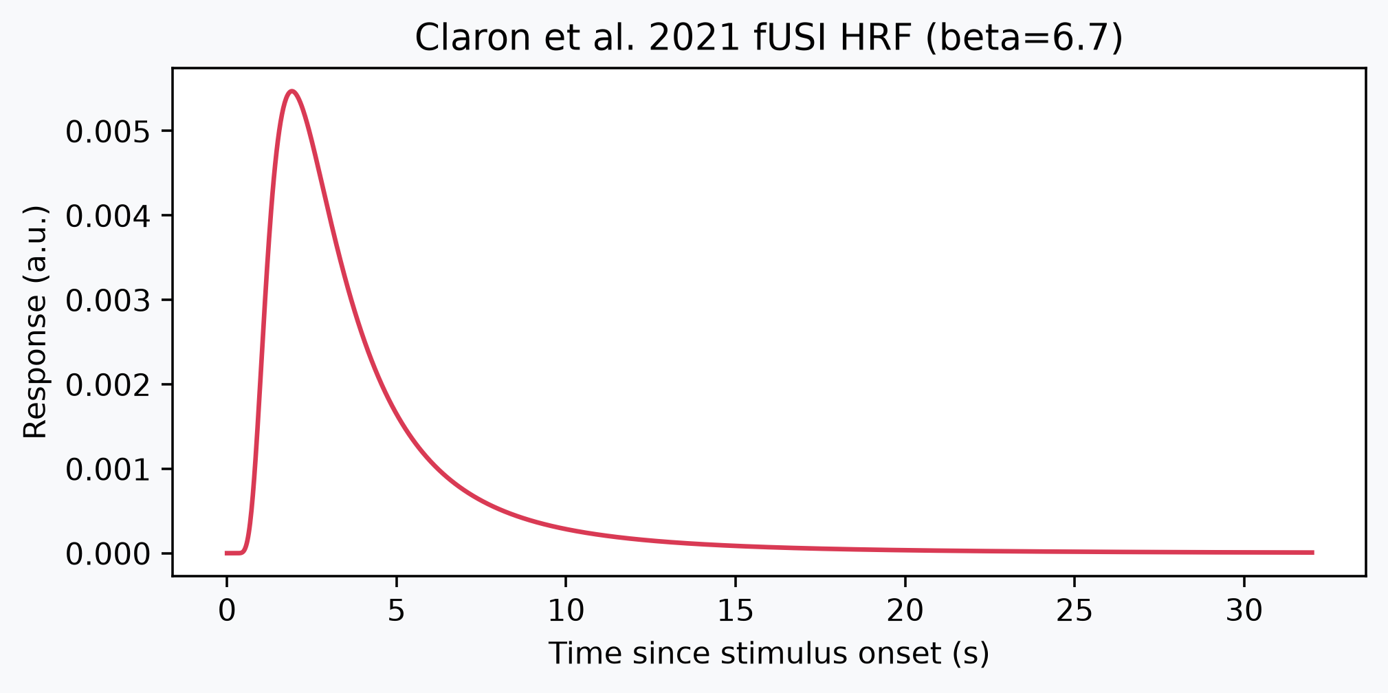
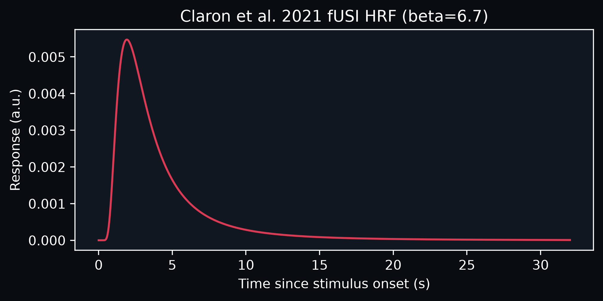
claron2021_hrf, an inverse-gamma HRF proposed for
functional ultrasound, rather than a canonical BOLD HRF. We tune its beta scale
parameter to 6.7 to obtain a faster peak response (around 2–3 seconds).
modified_claron2021 = partial(cf.glm.claron2021_hrf, beta=6.7)

# Sample the kernel on a fine grid to visualize its shape.
hrf_kernel = modified_claron2021(dt=1.0)
hrf_time = np.linspace(0, 32, len(hrf_kernel))

fig, ax = plt.subplots(figsize=(7, 3), facecolor=bg_color)
ax.plot(hrf_time, hrf_kernel, color="#d93a54")
ax.set_xlabel("Time since stimulus onset (s)")
ax.set_ylabel("Response (a.u.)")
_ = ax.set_title("Claron et al. 2021 fUSI HRF (beta=6.7)")
Model physiological noise with CompCor
Beyond the stimulus response, the signal contains structured nuisance fluctuations.
compute_compcor_confounds extracts the
leading principal components from a noise region—here the atlas "fiber tracts", that
ideally carries little task signal and global vascular fluctuations—and
we add them to the design as nuisance regressors (anatomical CompCor). We take three
components per run.
confounds = [
    cf.signal.compute_compcor_confounds(
        fusi,
        noise_mask=atlas.atlas.get_masks("fiber tracts")[0],
        n_components=3,
    )
    for fusi in resampled_fusi_list
]
Fit the first-level GLM
We hand the model specification to
FirstLevelModel up front: the HRF, the
"cosine" drift model that high-pass filters slow scanner/physiological drifts below
0.01 Hz, and the AR(1) noise model that accounts for temporal autocorrelation in the
residuals. fit then takes the runs
together with the events table and the per-run CompCor confounds, assembles a design
matrix for each run internally, and fits it to the data voxel by voxel. We apply a light
Gaussian spatial smoothing (0.3 mm FWHM per axis) to boost SNR and fit every voxel,
leaving the anatomical masking to the thresholding step below. Passing the list of runs
together combines them with a fixed-effects model.
glm = cf.glm.FirstLevelModel(
    smoothing_fwhm={"z": 0.3, "y": 0.3, "x": 0.3},
    hrf_model=modified_claron2021,
    drift_model="cosine",
    low_cutoff=0.01,
    noise_model="ar1",
)
glm.fit(resampled_fusi_list, events=events, confounds=confounds)
FirstLevelModel(hrf_model=functools.partial(<function claron2021_hrf at 0x7f2f1cf9ec40>, beta=6.7),
                smoothing_fwhm={'x': 0.3, 'y': 0.3, 'z': 0.3})
In a Jupyter environment, please rerun this cell to show the HTML representation or trust the notebook. On GitHub, the HTML representation is unable to render, please try loading this page with nbviewer.org.
Parameters
| hrf_model | functools.par...40>, beta=6.7) | |
| smoothing_fwhm | {'x': 0.3, 'y': 0.3, 'z': 0.3} | |
| drift_model | 'cosine' | |
| low_cutoff | 0.01 | |
| drift_order | 1 | |
| fir_delays | None | |
| noise_model | 'ar1' | |
| minimize_memory | True | |
| oversampling | 50 | |
| min_onset | -24.0 | |
| uniformity_tolerance | 0.01 | |
| mask | None |
Fitted attributes
| Name | Type | Value |
|---|---|---|
| design_matrices_ | list | [ acti...00 1.0 , acti...00 1.0 , acti...00 1.0 , acti...00 1.0 , ...] |
| results_ | list | [<confusius.gl...x7f2f1c3b34d0>, <confusius.gl...x7f2f70108770>, <confusius.gl...x7f2f1c0645f0>, <confusius.gl...x7f2f1c1e0d10>, ...] |
Inspect the design matrix
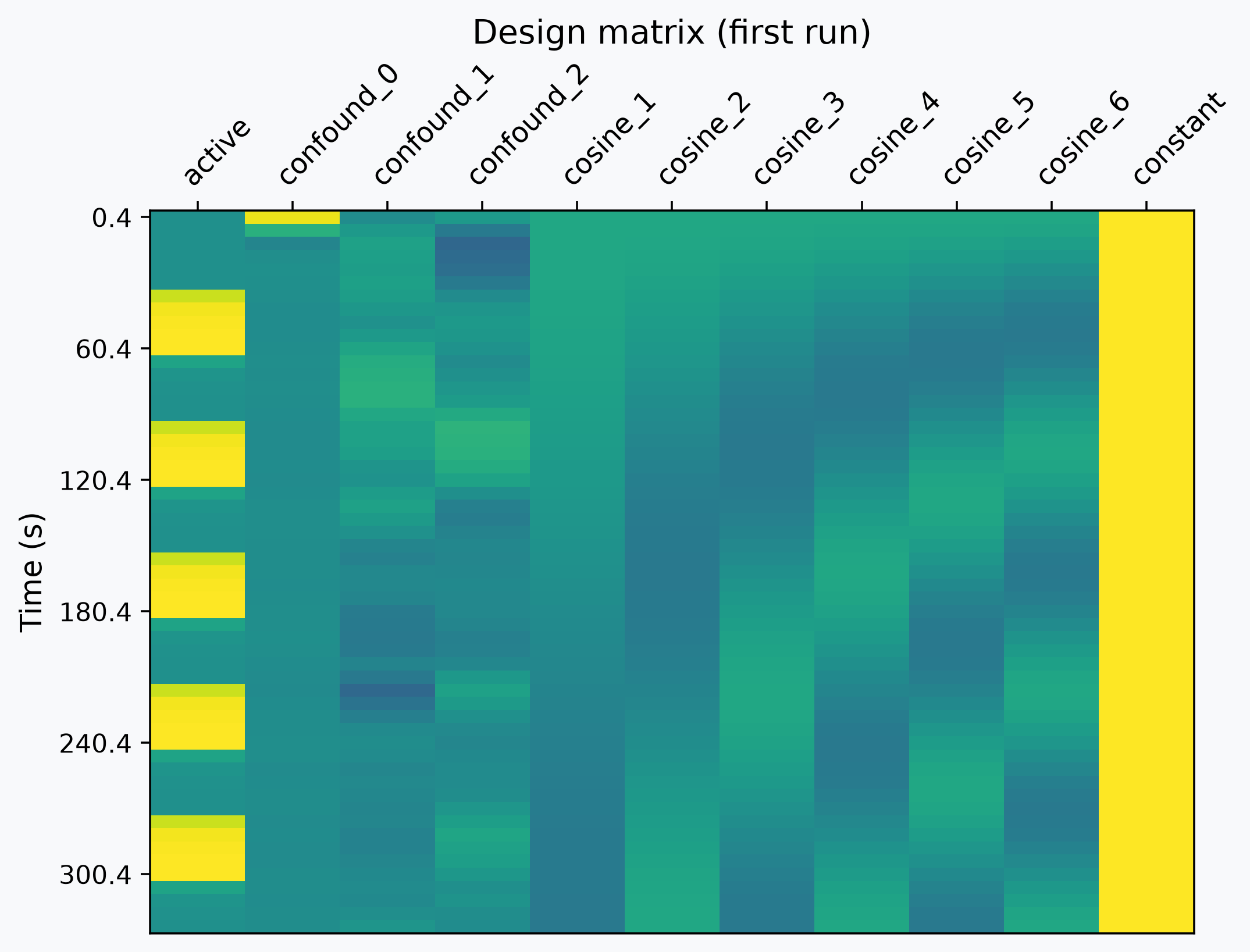
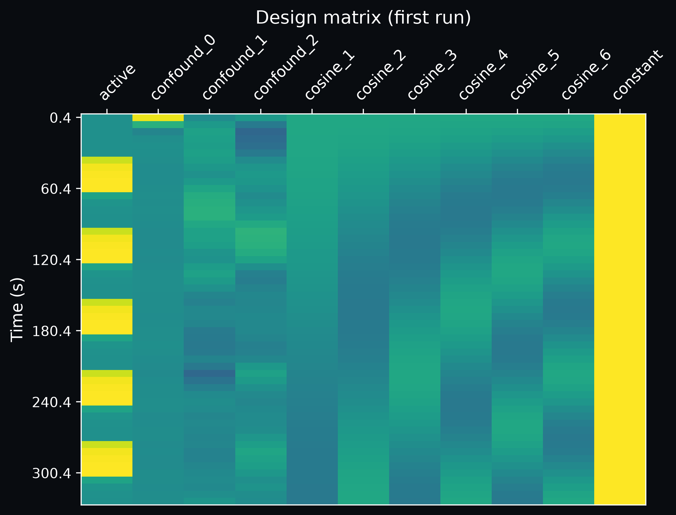
The fit assembled one design matrix per run (through
make_first_level_design_matrix) and
stored them on the fitted model as design_matrices_. Each run gets its own matrix
because its CompCor regressors are estimated from its own data. Pulling the first run's
matrix back out lets us see exactly what the model fit.
Visualizing that matrix makes the model concrete. Each column is a regressor and each
row a volume (time runs top to bottom). The leftmost active column shows the
HRF-convolved stimulation blocks; the CompCor and drift columns follow, and the constant
column models the baseline.
design_matrix = glm.design_matrices_[0]

_ = cf.plotting.plot_design_matrix(
    design_matrix,
    title="Design matrix (first run)",
    index_yaxis=True,
    bg_color=bg_color,
)
Compute and display the activation map
compute_contrast turns
the fitted model into a statistical map from a contrast: a weight vector over the
design-matrix columns. Before computing it, we can look at the contrast itself with
plot_contrast_matrix, which lays the
weights over the design regressors and makes explicit that the "active" contrast
simply selects the stimulation regressor while ignoring the CompCor, drift, and constant
nuisance columns.
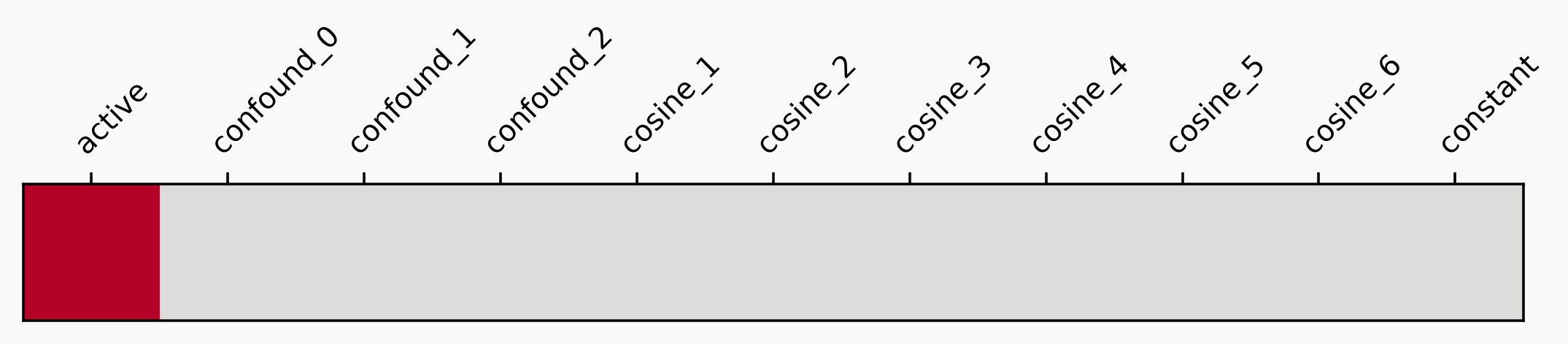
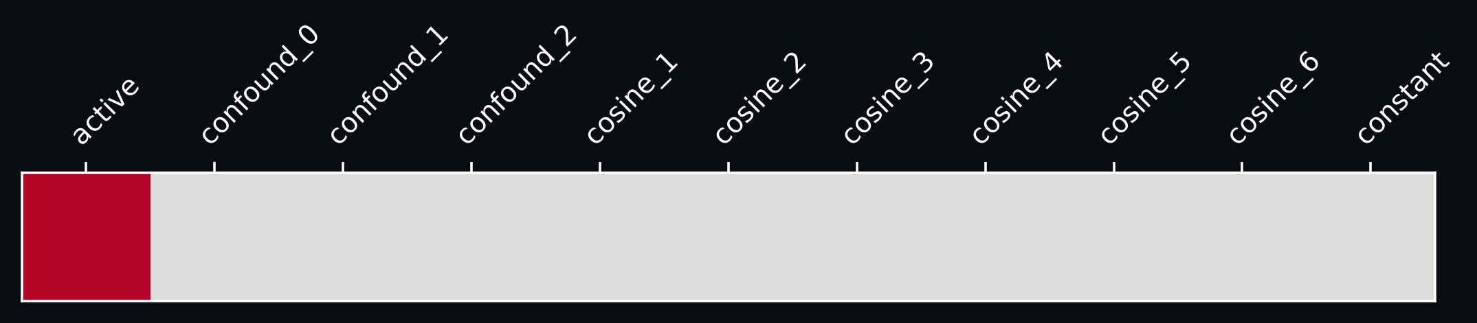
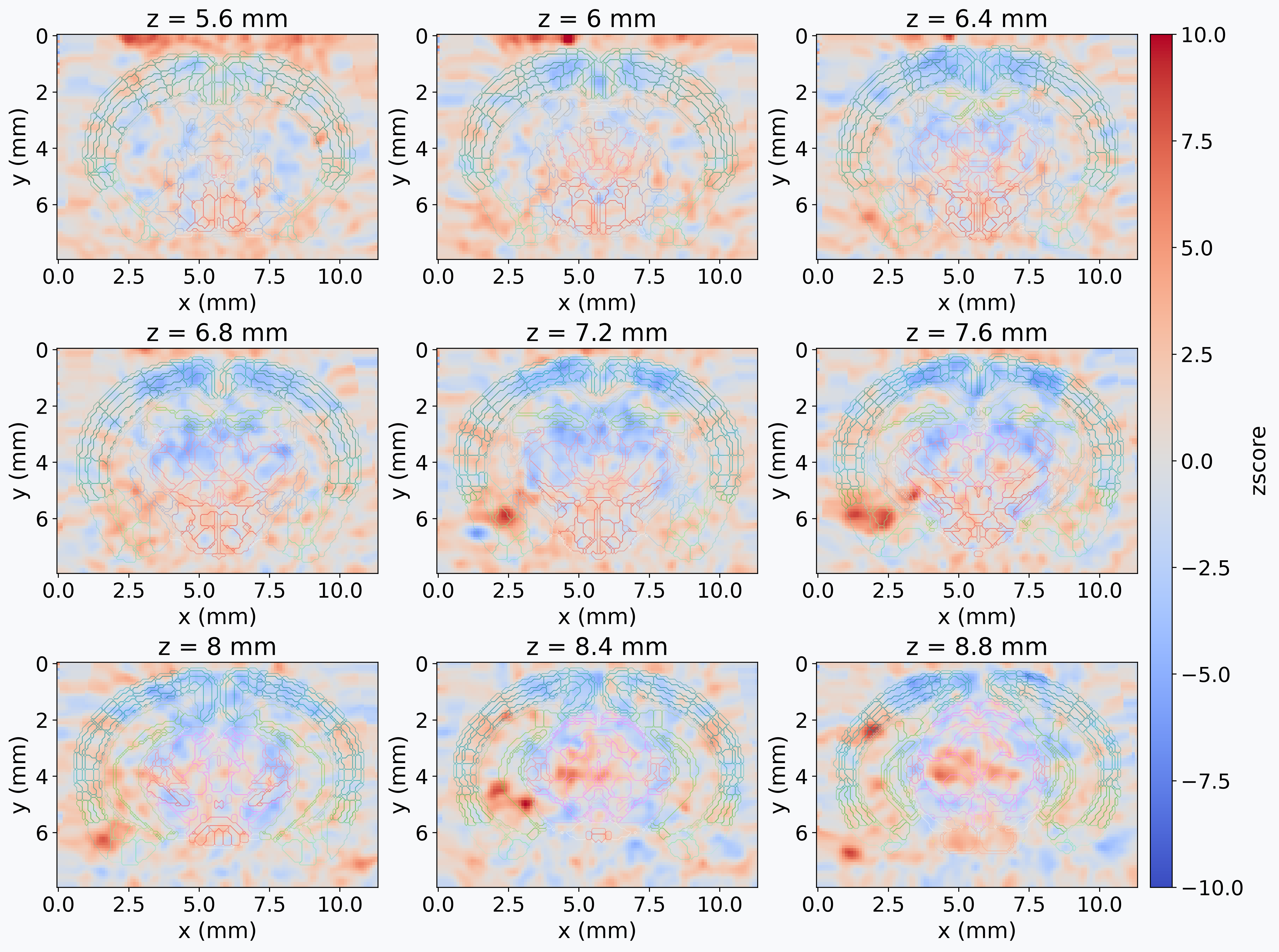
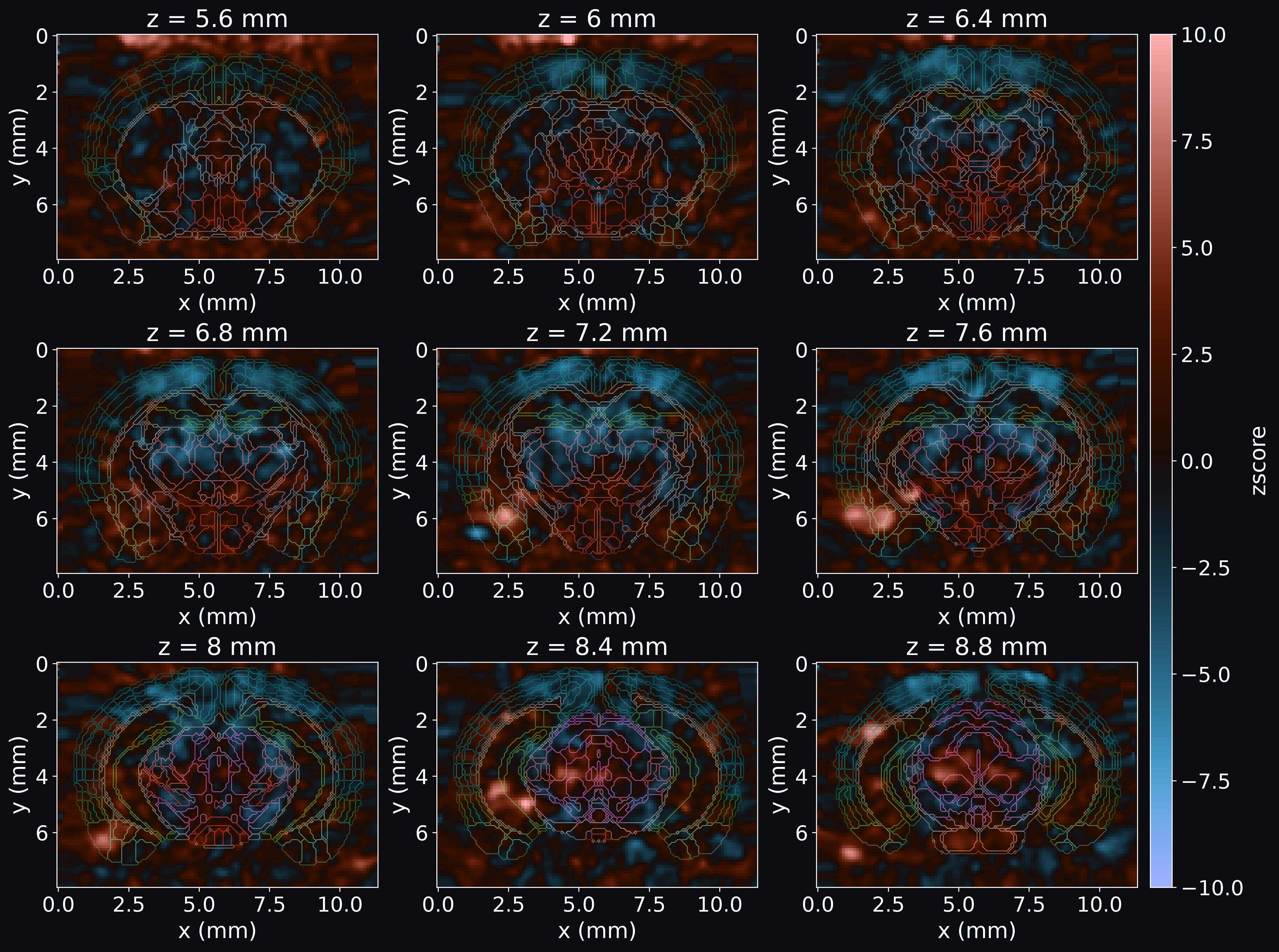
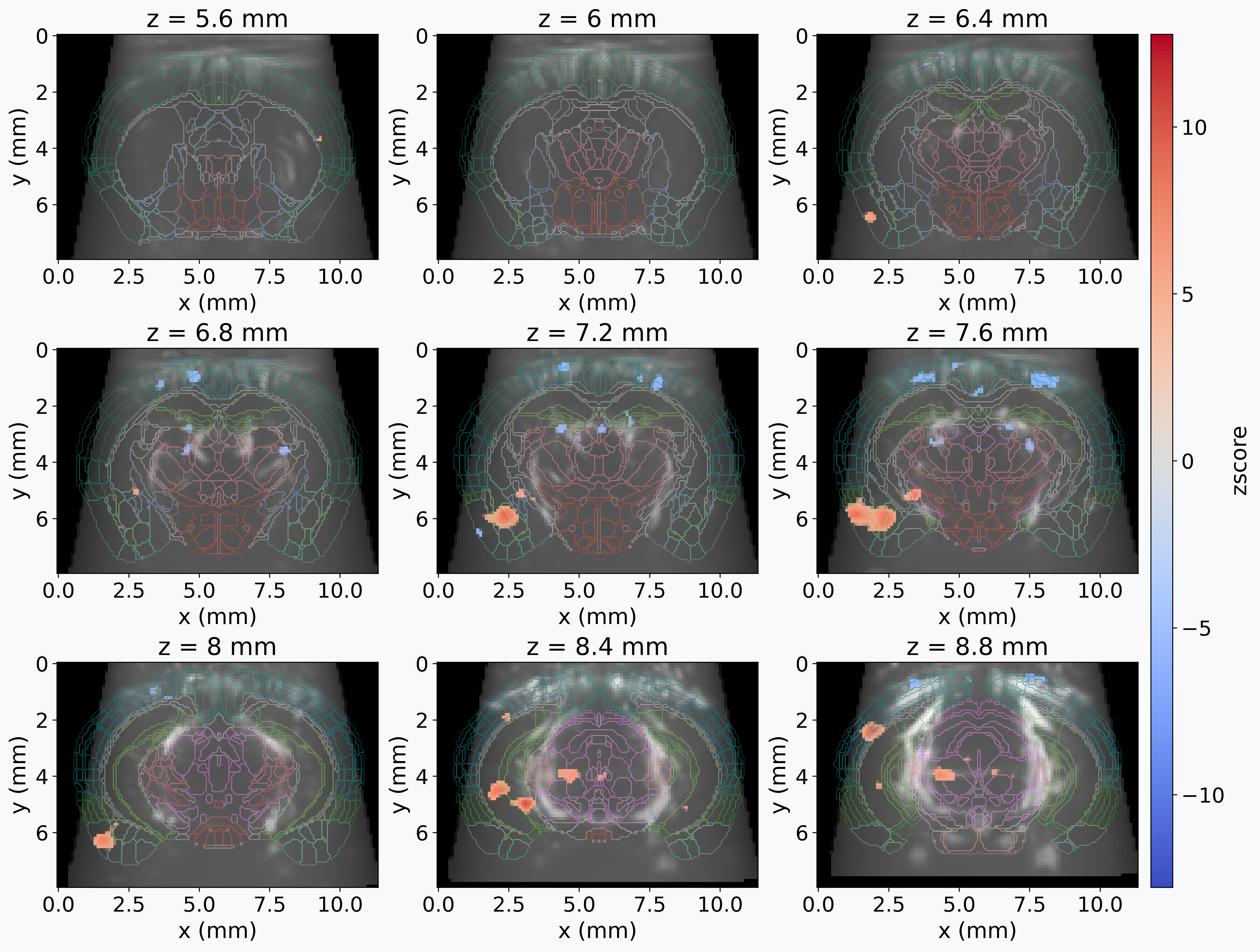
The "active" contrast then tests, at every voxel, whether that stimulation regressor
has a non-zero effect, and returns a z-score map. We display it over a range of atlas
slices with the region boundaries drawn on top for anatomical context.
z_score = glm.compute_contrast("active")

slice_coords = resampled_average_in_atlas.z[
    (resampled_average_in_atlas.z > 5.5) & (resampled_average_in_atlas.z < 9)
][::4]

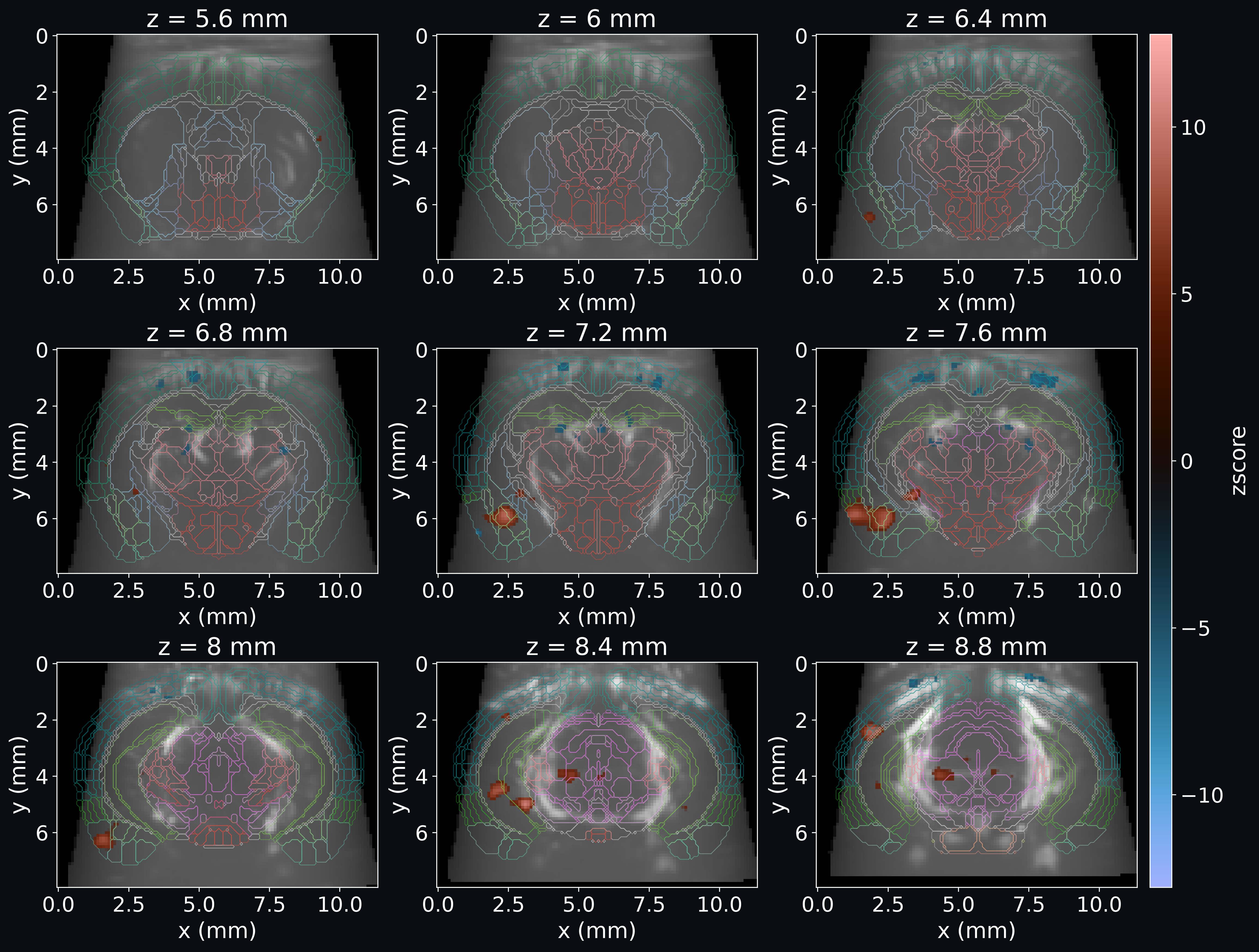
cmap = "berlin" if is_dark_theme else None
vmax = 10
fig = cf.plotting.plot_stat_map(
    z_score,
    slice_coords=slice_coords,
    nrows=3,
    vmax=vmax,
    bg_color=bg_color,
    cmap=cmap,
    fontsize=20,
)
_ = fig.add_contours(
    atlas.annotation,
    linewidths=0.6,
    slice_coords=slice_coords,
    alpha=0.4,
)
Threshold for statistical significance
The raw z-map shows the effect at every voxel; we might want to keep only those that are
statistically significant while controlling for the many thousands of simultaneous
tests. apply_statistical_threshold
applies a multiple-comparison correction (here Holm family-wise-error control at
alpha=0.01, restricted to the whole-brain "root" mask from the atlas), followed by
a cluster-extent threshold that drops surviving clusters smaller than 30 voxels. It
returns the map with the non-surviving voxels zeroed out, along with the z-value at
which the correction cut.
A hard threshold is not the only way to show significance. Rather than hiding the
sub-threshold voxels outright, we can let significance drive the opacity of the
overlay, which keeps the sub-threshold structure visible while still making the
significant clusters stand out. For that we convert the z-scores into two-sided
p-values and correct them with the same Holm procedure via
adjust_pvalues, which sets untested voxels (those
outside the mask) to 1.0. 1 - adjusted_p_values then gives an opacity scale
that we can hand to the plot as an alpha map.
thresholded_zscore, threshold = cf.stats.apply_statistical_threshold(
    z_score,
    mask=atlas.atlas.get_masks("root")[0],
    alpha=0.01,
    method="holm",
    cluster_threshold=30,
)

p_values = z_score.copy(deep=True)
p_values.values = np.clip(2.0 * sps.norm.sf(np.abs(z_score)), 0.0, 1.0)
adjusted_p_values = cf.stats.adjust_pvalues(
    p_values, mask=atlas.atlas.get_masks("root")[0], method="holm"
)
Explore the result interactively
The thresholded map, the anatomical reference, and the atlas labels can be loaded together into a napari viewer for 3D exploration:
Finally, we overlay the z-map on the mean power Doppler image (in dB) with the atlas contours, giving a single figure that places the odour response in its anatomical context.
fig = cf.plotting.plot_stat_map(
    z_score,
    bg_volume=resampled_average_in_atlas.fusi.scale.db(),
    slice_coords=slice_coords,
    nrows=3,
    bg_kwargs={"vmin": -20, "vmax": 0},
    bg_color=bg_color,
    alpha=1 - adjusted_p_values,
    cmap=cmap,
    fontsize=20,
)
_ = fig.add_contours(
    atlas.annotation,
    linewidths=0.6,
    slice_coords=slice_coords,
    alpha=0.4,
)
Total running time: 186.3 s