Visualization¶

ConfUSIus provides tools for both interactive exploration and static figure generation:

All functions accept DataArrays and use physical coordinates for axis scaling automatically. The Xarray accessor variants (.fusi.plot.*) offer a more concise syntax; both call the same underlying functions.

import csv

import confusius as cf
import numpy as np
from confusius.datasets import fetch_nunez_elizalde_2022
from napari.utils.colormaps import DirectLabelColormap


def _nunez_allen_label_colormap(structure_tree_csv, atlas_labels):
    """Build a napari labels colormap from structure-tree colors."""
    with open(structure_tree_csv, newline="", encoding="utf-8") as f:
        rows = list(csv.DictReader(f))

    labels = {int(v) for v in np.unique(atlas_labels.values) if int(v) > 0}
    key = max(
        ("graph_order", "sphinx_id", "id"),
        key=lambda k: len({int(float(r[k])) for r in rows if r.get(k)} & labels),
    )

    rgb = {}
    for r in rows:
        if not r.get(key) or not r.get("color_hex_triplet"):
            continue
        lab = int(float(r[key]))
        if lab not in labels:
            continue
        h = r["color_hex_triplet"].lstrip("#")
        rgb[lab] = tuple(int(h[i : i + 2], 16) / 255 for i in (0, 2, 4))

    return DirectLabelColormap(
        color_dict={
            0: np.zeros(4),
            None: np.zeros(4),
            **{k: np.array([*v, 0.7]) for k, v in rgb.items()},
        }
    )

bids_root = fetch_nunez_elizalde_2022(
    subjects=["CR022"],
    sessions=["20201011", "20201007"],
    tasks=["spontaneous"],
    acqs=["slice03"],
)

pwd = cf.load(
    bids_root
    / "sub-CR022/ses-20201011/fusi"
    / "sub-CR022_ses-20201011_task-spontaneous_acq-slice03_pwd.nii.gz"
)
mean_vol = pwd.mean("time").compute()
angio = cf.load(
    bids_root
    / "sub-CR022/ses-20201011/angio"
    / "sub-CR022_ses-20201011_pwd.nii.gz"
).compute()
angio_2 = cf.load(
    bids_root
    / "sub-CR022/ses-20201007/angio"
    / "sub-CR022_ses-20201007_pwd.nii.gz"
).compute()
atlas_labels = cf.load(
    bids_root
    / "derivatives/allenccf_align/sub-CR022/ses-20201011/fusi"
    / "sub-CR022_ses-20201011_space-fusi_desc-allenccf_dseg.nii.gz"
)
atlas_labels = atlas_labels.sel(z=mean_vol["z"], method="nearest").assign_coords(
    z=mean_vol["z"]
)

label_colormap = _nunez_allen_label_colormap(
    bids_root / "derivatives/allenccf_align/structure_tree_safe_2017.csv",
    atlas_labels,
)

Interactive Exploration with napari¶

ConfUSIus relies on napari for interactive visualization of 3D+t fUSI data. Napari handles large datasets efficiently through lazy loading, allowing you to explore even beamformed IQ data without running out of memory. You may find it helpful to read through the tour of the napari viewer to familiarize yourself with the controls and features.

Basic Usage¶

viewer, layer = pwd.fusi.plot.napari()

import confusius as cf

viewer, layer = cf.plotting.plot_napari(pwd)

This opens a napari viewer with a scale bar, colorbar, and correct physical scaling across axes. The viewer is fully interactive: you can zoom, pan, and scroll through time and elevation slices with the sliders or mouse wheel.

Napari Parameters¶

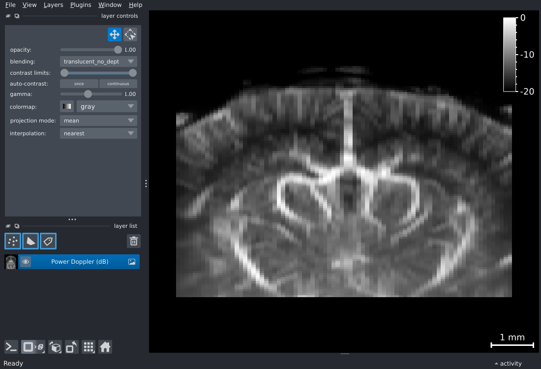
By default napari auto-scales contrast to the data range. For power Doppler, working in decibel scale with explicit limits is often more informative:

# dB-scaled power Doppler with fixed contrast window.
viewer, layer = cf.plotting.plot_napari(
    pwd.fusi.scale.db(),
    contrast_limits=(-20, 0),
    colormap="hot",
)

contrast_limits, colormap, and any other keyword arguments are forwarded directly to napari.imshow.

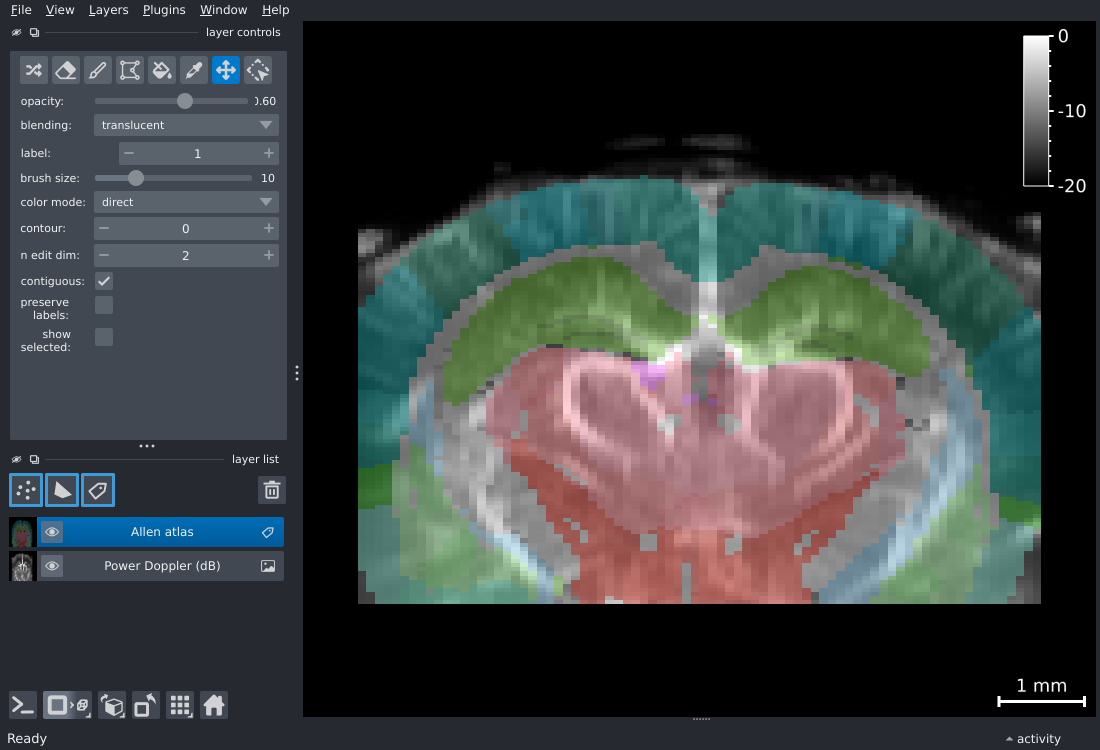
Overlaying an Atlas as a Labels Layer¶

Napari's labels layer renders integer-labeled masks as filled or contoured regions, ideal for visualizing an atlas alongside your power Doppler data. With the Nunez-Elizalde dataset, you can use the precomputed Allen segmentation in derivatives/allenccf_align:

import confusius as cf

# Load power Doppler mean volume and open viewer.
viewer, layer = cf.plotting.plot_napari(
    mean_vol.fusi.scale.db(),
    contrast_limits=(-20, 0),
)

# Add pre-registered Allen labels as a labels layer.
viewer, labels_layer = cf.plotting.plot_napari(
    atlas_labels,
    viewer=viewer,
    layer_type="labels",
    colormap=label_colormap,
    name="Allen atlas",
    opacity=0.6,
)

viewer, layer = pwd_before.fusi.plot.napari(name="Before correction")
viewer, layer = pwd_after.fusi.plot.napari(viewer=viewer, name="After correction")

Slicing Across Different Spatial Dimensions¶

By default, napari shows the last two spatial dimensions as a 2D plane and the remaining dimensions (e.g., time, z) as sliders. If you prefer a different default slicing axis—for example slicing along y (depth) instead of z (elevation)—use dim_order to reorder the spatial axes:

# Swap z and y: depth becomes the slider axis.
viewer, layer = pwd_3d.fusi.plot.napari(dim_order=("y", "z", "x"))

3D Rendering¶

For volumetric datasets, napari can render the data in full 3D using volume rendering (accessible by clicking the second icon in the bottom-left controls). In the 3D view you can drag to orbit, scroll to zoom, and use the napari controls to adjust the rendering.

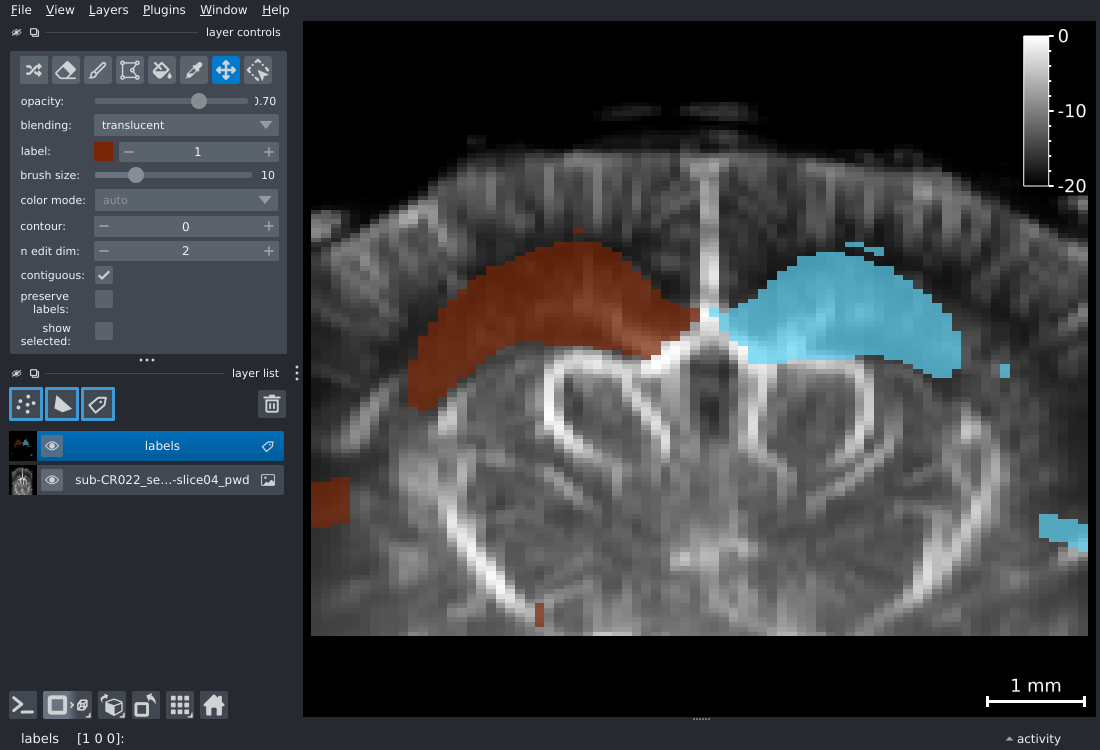
Manual ROI Drawing¶

draw_napari_labels opens a napari viewer with your data as a background image and an empty Labels layer on top. You can then paint integer labels directly in the viewer using napari's brush tool—each distinct integer becomes a separate region of interest (ROI).

import xarray as xr
import confusius as cf

pwd = cf.load("sub-01_task-awake_pwd.zarr")
mean_vol = pwd.mean("time").compute()

# Open viewer with an empty Labels layer ready for painting.
viewer, labels_layer = cf.plotting.draw_napari_labels(
    mean_vol.fusi.scale.db(),
    contrast_limits=(-20, 0),
    colormap="gray",
)

The Labels layer is aligned to the same physical coordinate frame as the image layer, so the spatial scale and origin are consistent regardless of voxel size or data origin.

Once you have finished painting, use labels_from_layer to convert the Labels layer into a stacked integer DataArray compatible with extract_with_labels, plot_contours, and VolumePlotter.add_contours:

from confusius.plotting import labels_from_layer

# Convert the painted layer to a stacked DataArray.
# label_map has dims ("masks", "z", "y", "x"), one layer per painted label.
label_map = labels_from_layer(labels_layer, mean_vol)

# Each label's color as painted in napari is stored in attrs["rgb_lookup"]
# and will be reused automatically by plot_contours and add_contours.

# Extract region-averaged signals.
region_signals = pwd.fusi.extract.with_labels(label_map)
# region_signals has dims (time, regions).

# Overlay contours on a volume plot.
plotter = mean_vol.fusi.scale.db().fusi.plot.volume(slice_mode="z", cmap="gray")
plotter.add_contours(label_map)

Static Volume Plots¶

plot_volume generates a static Matplotlib grid of 2D slices—one panel per coordinate along the chosen slicing dimension. It is the standard tool in ConfUSIus for generating static figures of 3D volumes, functional activation maps, or 3D angiography data.

Basic Usage¶

import xarray as xr
import confusius

pwd = cf.load("sub-01_task-awake_pwd.zarr")

# All elevation slices in an auto-sized grid.
plotter = pwd.fusi.plot.volume()

import xarray as xr
import confusius as cf

pwd = cf.load("sub-01_task-awake_pwd.zarr")

# All elevation slices in an auto-sized grid.
plotter = cf.plotting.plot_volume(pwd)

The function returns a VolumePlotter object that manages the underlying Matplotlib Figure and Axes and supports overlay operations (see Overlaying Contours).

When the data has multiple slices along the sliced dimension, plot_volume lays them out automatically in an approximately square grid:

angio = cf.load("sub-01_acq-angio_pwd.zarr")

plotter = angio.fusi.plot.volume(slice_mode="z", show_colorbar=False)

Selecting Slices and Colormap¶

By default all coordinates along slice_mode are shown. Use slice_coords to pick specific ones and cmap/vmin/vmax to control the colormap and contrast. The grid layout can be controlled using nrows and ncols, or by specifying axes directly with axes (see the API reference for details).

import numpy as np

z = angio["z"].values
margin = max(1, int(round(0.12 * (len(z) - 1))))
slice_coords = tuple(np.linspace(float(z[margin]), float(z[-margin - 1]), 3))

plotter = angio.fusi.scale.db().fusi.plot.volume(
    nrows=1,
    slice_mode="z",
    slice_coords=slice_coords,
    cmap="inferno",
    vmin=-20,
    vmax=0,
    show_colorbar=False,
)

Thresholding¶

For functional activation maps or data where you want to suppress noise, threshold sets a cutoff value. Subthreshold voxels are rendered transparently:

# Hide values where |data| < 3.0 (noise floor suppression).
plotter = stat_map.fusi.plot.volume(
    slice_mode="z",
    threshold=3.0,
    threshold_mode="lower",
    cmap="RdBu_r",
    vmin=-6,
    vmax=6,
)

threshold_mode="upper" masks values above the threshold instead—useful for removing saturation artifacts or thresholding decibel-scaled data.

Saving and Closing¶

plotter = pwd.fusi.plot.volume(slice_mode="z", cmap="hot")
plotter.savefig("sub-01_task-awake_pwd.png", dpi=150)
plotter.close()

Pass any keyword argument accepted by matplotlib.figure.Figure.savefig (e.g., bbox_inches="tight", transparent=True).

Overlaying Contours¶

Atlas outlines or region of interest (ROI) boundaries can be drawn on top of a volume plot to provide anatomical context. ConfUSIus represents masks as integer-labeled DataArrays where 0 is background and each positive integer identifies a distinct region.

Contours on top of a Volume¶

The most common use case is to draw atlas outlines on top of a fUSI volume. plot_volume returns a VolumePlotter that remembers the coordinate-to-axis mapping; calling add_contours on it draws outlines on the matching panels. Masks produced by Atlas.get_masks carry Allen colors in their attrs["rgb_lookup"], so no explicit color argument is needed:

from confusius.atlas import Atlas

# Load Atlas and resample to fUSI space (see Registration guide).
atlas = Atlas.from_brainglobe("allen_mouse_100um")
atlas_fusi = atlas.resample_like(mean_vol, transform)

# Step 1: display an average power Doppler volume.
plotter = cf.plotting.plot_volume(
    pwd.fusi.scale.db(),
    slice_mode="z",
    cmap="gray",
    vmin=-20,
    vmax=0,
    cbar_label="Power Doppler (dB)",
)

# Step 2: overlay contours. Allen colors are read from atlas_mask.attrs["rgb_lookup"]
# automatically.
plotter.add_contours(atlas_fusi.annotation)

Coordinate matching is done in physical units, matching contour coordinates with those of the previously plotted volume. Slices present in the mask but absent from the volume are skipped with a warning.

Contours-only Grid¶

plot_contours produces a contour grid without any background image—useful for quickly inspecting mask or atlas coverage across slices, or for drawing contours onto a set of pre-existing Axes without the coordinate-matching of VolumePlotter:

# Contours on a black background (default).
plotter = cf.plotting.plot_contours(atlas_fusi.annotation, slice_mode="z")

# Specific colors per region.
plotter = cf.plotting.plot_contours(
    atlas_fusi.annotation,
    slice_mode="z",
    colors={1: "cyan", 2: "magenta"},
)

The .fusi.plot.contours() accessor provides the same function with a shorter syntax:

plotter = atlas_fusi.annotation.fusi.plot.contours(slice_mode="z")

Composite Plots¶

plot_composite overlays two volumes as a red/cyan composite: the first volume drives the red channel, the second drives the cyan channel (green + blue). This is the same encoding used by the live registration progress preview and is a quick way to inspect how well two volumes are aligned: two sessions of the same subject, a moving image against a reference, or a registered output against its target.

Basic Usage¶

# Every third elevation slice keeps the figure compact while still showing the
# anatomical depth range.
composite_slices = list(np.asarray(angio["z"].values, dtype=float)[::3][:-1])

# Two angiography volumes from different sessions of the same subject.
plotter = angio.fusi.plot.composite(
    angio_2, slice_coords=composite_slices, normalize_strategy="per_slice"
)

# Every third elevation slice keeps the figure compact while still showing the
# anatomical depth range.
composite_slices = list(np.asarray(angio["z"].values, dtype=float)[::3][:-1])

# Two angiography volumes from different sessions of the same subject.
plotter = cf.plotting.plot_composite(
    angio, angio_2, slice_coords=composite_slices, normalize_strategy="per_slice"
)

By default angio_2 is resampled onto angio's grid (resample=True), so the two volumes do not need to share the same coordinates. Additionally, the function returns a VolumePlotter so you can use add_contours to layer atlas outlines over the composite.

Normalization Strategies¶

normalize_strategy controls how voxel intensities are mapped into the [0, 1] range that drives each channel:

Skipping Resampling¶

If the two volumes already share the same grid (if one was previously registered onto the other) pass resample=False to skip the resample step:

plotter = fixed.fusi.plot.composite(registered_moving, resample=False)

When resample=False, the two arrays must share dimensions, shape, and coordinates within tolerance. Coordinates are checked with numpy.allclose-style tolerances (rtol=1e-5, atol=1e-8 by default); once the check passes, data2's coordinates are replaced with data1's so the two volumes share an exact coordinate frame downstream. Widen rtol / atol to accept acquisitions on offset grids that you know are equivalent.

Carpet Plots¶

A carpet plot (also called a grayplot or Power plot¹) displays every voxel's time-series as a row in a 2D raster image with time on the x-axis. Z-scored by default, it makes motion artifacts, global signal transients, and outlier volumes immediately visible as vertical stripes or abrupt intensity changes.

Carpet plots are primarily used for quality control—for a deeper discussion of QC metrics, see the Quality Control guide.

Basic Usage¶

import xarray as xr
import confusius

brain_mask = cf.load("brain_mask.zarr")

fig, ax = pwd.fusi.plot.carpet(mask=brain_mask)

import xarray as xr
import confusius as cf

brain_mask = cf.load("brain_mask.zarr")

fig, ax = cf.plotting.plot_carpet(pwd, mask=brain_mask)

Without a mask, all non-zero voxels are included. With a mask, only voxels where mask == True (or mask > 0 for integer-labeled masks) are shown. See the API reference of plot_carpet for more options.

Next Steps¶

Now that you can visualize your data, you're ready for:

1. Registration: Correct for motion and align acquisitions to an anatomical template.
2. Quality Control: Assess data quality and identify artifacts.
3. Signal Processing: Extract regional signals and apply denoising.

API Reference¶

For full parameter documentation, see the Plotting API reference and the Xarray Integration API reference.