Create a fUSI DataArray from a MAT file
This example downloads a power Doppler MAT file from the public dataset accompanying
Rabut et al. (2024)1 and wraps it
in a ConfUSIus DataArray with
create_fusi_dataarray.
Since MAT files can contain any custom data, ConfUSIus cannot read them directly. The point of this example is to show the shortest path from a lab-specific MAT file array plus metadata to the standard ConfUSIus DataArray representation. This example then reproduces figure 4D from Rabut et al. (2024) using a simple general linear model.
from functools import partial
from pathlib import Path

import h5py
import matplotlib as mpl
import matplotlib.pyplot as plt
import numpy as np
import pandas as pd
import pooch
import xarray as xr
from remotezip import RemoteZip

import confusius as cf
from confusius.glm import FirstLevelModel, gamma_hrf

# Adapt colors to the current Matplotlib style.
bg_color = mpl.colors.to_hex(mpl.rcParams["figure.facecolor"])
is_dark_theme = sum(mpl.colors.to_rgb(bg_color)) / 3 < 0.5
stat_cmap = "berlin" if is_dark_theme else None

# Keep notebook output compact for large DataArray displays.
_ = xr.set_options(display_expand_attrs=False, display_expand_data=False)
Download one recording from the Rabut et al. (2024) dataset
The Caltech record stores all data in a single ZIP archive. We extract a single MAT file from the archive to avoid downloading the full dataset. The MAT file contains a power Doppler recording of a human subject performing a simple task, with accompanying timestamps, task labels, and ultrasound metadata.
RECORD_URL = "https://data.caltech.edu/api/records/f3y3k-em558/files/data.zip/content"
RECORD_DOI = "https://doi.org/10.22002/f3y3k-em558"
MEMBER = "data/human/S2R1.mat"

cache_dir = Path(pooch.os_cache("confusius")) / "rabut_2024_human_glm"
cache_dir.mkdir(parents=True, exist_ok=True)
mat_path = cache_dir / Path(MEMBER).name

if not mat_path.exists():
    with RemoteZip(RECORD_URL) as archive:
        with archive.open(MEMBER) as source, mat_path.open("wb") as target:
            target.write(source.read())
Load the power Doppler array and metadata
This MAT file v7.3 is HDF5-backed, so we use [h5py.File][] to open it. We
transpose the Doppler array to (time, y, x) and flip the lateral axis to match the
orientation of the original paper figures.
with h5py.File(mat_path, "r") as mat:
    doppler = np.flip(mat["dop"][()].astype("float32").transpose(0, 2, 1), axis=2)
    task = mat["task"][:, 0].astype("float32")
    timestamps = mat["timestamps"][0]
    wavelength = float(mat["UF/Lambda"][0, 0])
    run_label = "".join(map(chr, mat["run_label"][()].ravel().astype(int))).strip()

print(run_label)
print(f"Data shape: {doppler.shape}")
Wrap the raw array with [create_fusi_dataarray][cf.create_fusi_dataarray]
After transposing the MATLAB array, the Doppler movie is (time, y, x). ConfUSIus
adds the missing singleton z axis and returns the canonical (time, z, y, x)
layout. The timestamps have small acquisition jitter, so we pass them as an exact
coordinate. Following the authors' analysis code, we use the acoustic wavelength from
UF.Lambda for axial spacing and the 0.3 mm probe pitch for lateral spacing. We keep
depths between 10 and 30 mm to focus on the part of the image with good SNR.
dy = wavelength
dx = 0.3
y = dy / 2 + np.arange(doppler.shape[1]) * dy
x = dx / 2 + np.arange(doppler.shape[2]) * dx

power_doppler = cf.create_fusi_dataarray(
    doppler,
    dims=("time", "y", "x"),
    coords={"time": timestamps, "y": y, "x": x},
    dz=1.0,
    name="power_doppler",
    attrs={"source": RECORD_DOI, "source_member": MEMBER},
).sel(y=slice(10, 30))

time_step = float(np.median(np.diff(timestamps)))
power_doppler = cf.timing.resample_to_uniform_time(power_doppler, step=time_step)
task_da = xr.DataArray(task, dims="time", coords={"time": timestamps})
task_da = cf.timing.resample_to_uniform_time(
    task_da,
    start=float(power_doppler.time[0]),
    stop=float(power_doppler.time[-1]),
    step=time_step,
    method="nearest",
)
power_doppler
- time: 270
- z: 1
- y: 97
- x: 128
- 2.106e+11 2.707e+11 3.04e+11 ... 2.945e+11 2.652e+11 2.58e+11
array([[[[2.10577752e+11, 2.70662992e+11, 3.04037921e+11, ..., 1.40320457e+11, 1.24857090e+11, 1.24517777e+11], [2.14506717e+11, 2.85069410e+11, 3.43384588e+11, ..., 1.39885674e+11, 1.25527794e+11, 1.19126106e+11], [2.28316201e+11, 2.33571320e+11, 2.40582951e+11, ..., 1.35647912e+11, 1.29280238e+11, 1.03471677e+11], ..., [2.79672553e+11, 3.12990728e+11, 3.13475138e+11, ..., 2.91363127e+11, 2.69979779e+11, 2.63551336e+11], [2.83264451e+11, 2.91544793e+11, 2.94284689e+11, ..., 3.15664105e+11, 3.20567771e+11, 2.88501793e+11], [2.64020197e+11, 3.03924871e+11, 2.98198532e+11, ..., 3.05831346e+11, 2.91014967e+11, 2.96275345e+11]]], [[[2.40716352e+11, 2.83655943e+11, 2.91034403e+11, ..., 1.40351818e+11, 1.28603264e+11, 1.16492990e+11], [2.23595700e+11, 2.71761266e+11, 3.31479128e+11, ..., 1.50428025e+11, 1.35002079e+11, 1.19212331e+11], [2.60899869e+11, 2.21150151e+11, 2.92841696e+11, ..., ... [2.65342913e+11, 2.97345883e+11, 3.04962160e+11, ..., 3.06916498e+11, 2.83746202e+11, 2.60658780e+11], [3.05788289e+11, 3.07075603e+11, 2.99803367e+11, ..., 3.13945462e+11, 2.89581501e+11, 2.67835313e+11]]], [[[2.67361939e+11, 2.70543169e+11, 2.89336457e+11, ..., 1.52472939e+11, 1.36244835e+11, 1.19496068e+11], [1.91441988e+11, 2.21729586e+11, 2.77770194e+11, ..., 1.55218769e+11, 1.39294126e+11, 1.27337899e+11], [1.93200875e+11, 2.30568764e+11, 2.62727546e+11, ..., 1.46543792e+11, 1.28960110e+11, 1.17371700e+11], ..., [2.76503547e+11, 2.92960119e+11, 3.06788047e+11, ..., 2.80144034e+11, 2.67253181e+11, 2.87594611e+11], [2.90532280e+11, 2.77860583e+11, 3.09633139e+11, ..., 2.86310089e+11, 2.79444401e+11, 2.55675877e+11], [2.93681132e+11, 3.02512800e+11, 3.20574481e+11, ..., 2.94487661e+11, 2.65201840e+11, 2.58004634e+11]]]], shape=(270, 1, 97, 128)) - time(time)float640.0 1.614 3.228 ... 432.6 434.2
- units :
- s
- volume_acquisition_reference :
- start
- volume_acquisition_duration :
- 1.613999999994121
array([ 0. , 1.614, 3.228, ..., 430.938, 432.552, 434.166], shape=(270,))
- z(z)float640.0
- units :
- mm
- voxdim :
- 1.0
array([0.])
- y(y)float6410.16 10.37 10.57 ... 29.67 29.88
- units :
- mm
- voxdim :
- 0.2053333333333338
array([10.164 , 10.369333, 10.574667, 10.78 , 10.985333, 11.190667, 11.396 , 11.601333, 11.806667, 12.012 , 12.217333, 12.422667, 12.628 , 12.833333, 13.038667, 13.244 , 13.449333, 13.654667, 13.86 , 14.065333, 14.270667, 14.476 , 14.681333, 14.886667, 15.092 , 15.297333, 15.502667, 15.708 , 15.913333, 16.118667, 16.324 , 16.529333, 16.734667, 16.94 , 17.145333, 17.350667, 17.556 , 17.761333, 17.966667, 18.172 , 18.377333, 18.582667, 18.788 , 18.993333, 19.198667, 19.404 , 19.609333, 19.814667, 20.02 , 20.225333, 20.430667, 20.636 , 20.841333, 21.046667, 21.252 , 21.457333, 21.662667, 21.868 , 22.073333, 22.278667, 22.484 , 22.689333, 22.894667, 23.1 , 23.305333, 23.510667, 23.716 , 23.921333, 24.126667, 24.332 , 24.537333, 24.742667, 24.948 , 25.153333, 25.358667, 25.564 , 25.769333, 25.974667, 26.18 , 26.385333, 26.590667, 26.796 , 27.001333, 27.206667, 27.412 , 27.617333, 27.822667, 28.028 , 28.233333, 28.438667, 28.644 , 28.849333, 29.054667, 29.26 , 29.465333, 29.670667, 29.876 ]) - x(x)float640.15 0.45 0.75 ... 37.95 38.25
- units :
- mm
- voxdim :
- 0.3000000000000007
array([ 0.15,  0.45,  0.75,  1.05,  1.35,  1.65,  1.95,  2.25,  2.55,  2.85,
        3.15,  3.45,  3.75,  4.05,  4.35,  4.65,  4.95,  5.25,  5.55,  5.85,
        6.15,  6.45,  6.75,  7.05,  7.35,  7.65,  7.95,  8.25,  8.55,  8.85,
        9.15,  9.45,  9.75, 10.05, 10.35, 10.65, 10.95, 11.25, 11.55, 11.85,
       12.15, 12.45, 12.75, 13.05, 13.35, 13.65, 13.95, 14.25, 14.55, 14.85,
       15.15, 15.45, 15.75, 16.05, 16.35, 16.65, 16.95, 17.25, 17.55, 17.85,
       18.15, 18.45, 18.75, 19.05, 19.35, 19.65, 19.95, 20.25, 20.55, 20.85,
       21.15, 21.45, 21.75, 22.05, 22.35, 22.65, 22.95, 23.25, 23.55, 23.85,
       24.15, 24.45, 24.75, 25.05, 25.35, 25.65, 25.95, 26.25, 26.55, 26.85,
       27.15, 27.45, 27.75, 28.05, 28.35, 28.65, 28.95, 29.25, 29.55, 29.85,
       30.15, 30.45, 30.75, 31.05, 31.35, 31.65, 31.95, 32.25, 32.55, 32.85,
       33.15, 33.45, 33.75, 34.05, 34.35, 34.65, 34.95, 35.25, 35.55, 35.85,
       36.15, 36.45, 36.75, 37.05, 37.35, 37.65, 37.95, 38.25])
- source :
- https://doi.org/10.22002/f3y3k-em558
- source_member :
- data/human/S2R1.mat
Plot the mean power Doppler image
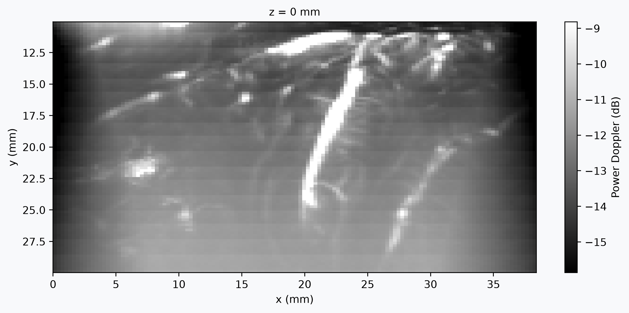
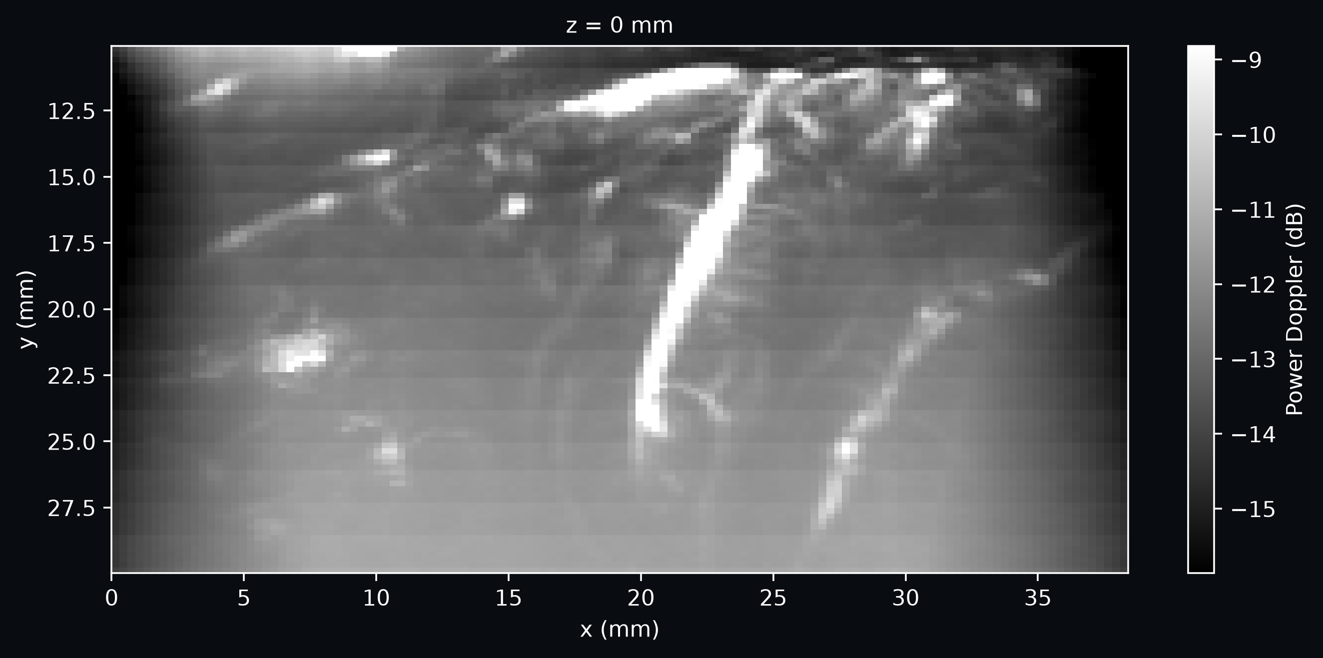
Once the custom file is represented as a DataArray, ConfUSIus plotting helpers work the same way as they do for built-in loaders.
mean_doppler = power_doppler.mean("time").fusi.scale.db()
plotter = mean_doppler.fusi.plot.volume(
    cbar_label="Power Doppler (dB)",
    bg_color=bg_color,
)
Motion-correct, smooth, and fit a simple task GLM
The paper reports rigid-body motion correction, 2D Gaussian spatial smoothing, temporal smoothing, detrending, and baseline scaling before the GLM. We reproduce all of these steps with ConfUSIus below.
# The default learning rate is conservative; for this recording, 1.0 recovers the motion
# better.
registered = power_doppler.fusi.register.volumewise(learning_rate=1.0)

# The paper reports a 2D Gaussian smoothing kernel with FWHM = 0.471 mm in both
# spatial dimensions.
smoothed = cf.spatial.smooth_volume(registered, fwhm=0.471)

# The paper reports a simple moving average for temporal smoothing.
filtered = smoothed.rolling(time=6, min_periods=1).mean()

# The paper reports baseline scaling to percent signal change relative to the mean of
# the rest blocks.
baseline = filtered.where(task_da == 0).mean("time")
scaled = 100 * filtered / baseline

time_values = power_doppler.time.values
edges = np.diff(np.r_[0.0, task_da.values, 0.0])
starts = np.flatnonzero(edges == 1.0)
stops = np.flatnonzero(edges == -1.0)
stop_times = np.r_[time_values, time_values[-1] + time_step][stops]
events = pd.DataFrame(
    {
        "onset": time_values[starts],
        "duration": stop_times - time_values[starts],
        "trial_type": "task",
    }
)


# We handle slow drift in FirstLevelModel with a cosine drift model. The task regressor
# is convolved with the single-gamma human fUSI HRF reported in the paper (`τ = 0.7`, `δ
# = 3 s`, `n = 3`).
tau = 0.7
n = 3
human_fusi_hrf = partial(
    gamma_hrf,
    time_length=16.0,
    peak_delay=(n - 1) * tau,
    dispersion=tau,
    onset=3.0,
)

model = FirstLevelModel(
    hrf_model=human_fusi_hrf, noise_model="ols", drift_model="cosine", low_cutoff=0.002
)
model.fit(scaled, events=events)

z_map = model.compute_contrast("task")
z_map
- z: 1
- y: 97
- x: 128
- -3.894 -3.584 -3.501 -3.76 -3.985 ... -8.179 -10.94 -13.72 -12.56
array([[[ -3.8937532 , -3.58374388, -3.50061825, ..., -8.74608067, -7.7934519 , -6.9910038 ], [ -1.51661246, -1.08157347, -0.89801277, ..., -7.08660289, -5.89104405, -4.75516857], [ 2.85558461, 3.98647903, 3.89770414, ..., -4.53545928, -4.30102831, -3.78234729], ..., [ 1.85772468, 3.81929143, 6.30793229, ..., -9.40418916, -12.4964886 , -12.27100517], [ 1.80686747, 3.91859188, 5.8298708 , ..., -10.92740815, -13.19299524, -12.42946417], [ 1.52253385, 3.68687158, 4.26127411, ..., -10.94084381, -13.72436736, -12.56125728]]], shape=(1, 97, 128)) - z(z)float640.0
- units :
- mm
- voxdim :
- 1.0
array([0.])
- y(y)float6410.16 10.37 10.57 ... 29.67 29.88
- units :
- mm
- voxdim :
- 0.2053333333333338
array([10.164 , 10.369333, 10.574667, 10.78 , 10.985333, 11.190667, 11.396 , 11.601333, 11.806667, 12.012 , 12.217333, 12.422667, 12.628 , 12.833333, 13.038667, 13.244 , 13.449333, 13.654667, 13.86 , 14.065333, 14.270667, 14.476 , 14.681333, 14.886667, 15.092 , 15.297333, 15.502667, 15.708 , 15.913333, 16.118667, 16.324 , 16.529333, 16.734667, 16.94 , 17.145333, 17.350667, 17.556 , 17.761333, 17.966667, 18.172 , 18.377333, 18.582667, 18.788 , 18.993333, 19.198667, 19.404 , 19.609333, 19.814667, 20.02 , 20.225333, 20.430667, 20.636 , 20.841333, 21.046667, 21.252 , 21.457333, 21.662667, 21.868 , 22.073333, 22.278667, 22.484 , 22.689333, 22.894667, 23.1 , 23.305333, 23.510667, 23.716 , 23.921333, 24.126667, 24.332 , 24.537333, 24.742667, 24.948 , 25.153333, 25.358667, 25.564 , 25.769333, 25.974667, 26.18 , 26.385333, 26.590667, 26.796 , 27.001333, 27.206667, 27.412 , 27.617333, 27.822667, 28.028 , 28.233333, 28.438667, 28.644 , 28.849333, 29.054667, 29.26 , 29.465333, 29.670667, 29.876 ]) - x(x)float640.15 0.45 0.75 ... 37.95 38.25
- units :
- mm
- voxdim :
- 0.3000000000000007
array([ 0.15,  0.45,  0.75,  1.05,  1.35,  1.65,  1.95,  2.25,  2.55,  2.85,
        3.15,  3.45,  3.75,  4.05,  4.35,  4.65,  4.95,  5.25,  5.55,  5.85,
        6.15,  6.45,  6.75,  7.05,  7.35,  7.65,  7.95,  8.25,  8.55,  8.85,
        9.15,  9.45,  9.75, 10.05, 10.35, 10.65, 10.95, 11.25, 11.55, 11.85,
       12.15, 12.45, 12.75, 13.05, 13.35, 13.65, 13.95, 14.25, 14.55, 14.85,
       15.15, 15.45, 15.75, 16.05, 16.35, 16.65, 16.95, 17.25, 17.55, 17.85,
       18.15, 18.45, 18.75, 19.05, 19.35, 19.65, 19.95, 20.25, 20.55, 20.85,
       21.15, 21.45, 21.75, 22.05, 22.35, 22.65, 22.95, 23.25, 23.55, 23.85,
       24.15, 24.45, 24.75, 25.05, 25.35, 25.65, 25.95, 26.25, 26.55, 26.85,
       27.15, 27.45, 27.75, 28.05, 28.35, 28.65, 28.95, 29.25, 29.55, 29.85,
       30.15, 30.45, 30.75, 31.05, 31.35, 31.65, 31.95, 32.25, 32.55, 32.85,
       33.15, 33.45, 33.75, 34.05, 34.35, 34.65, 34.95, 35.25, 35.55, 35.85,
       36.15, 36.45, 36.75, 37.05, 37.35, 37.65, 37.95, 38.25])
- source :
- https://doi.org/10.22002/f3y3k-em558
- source_member :
- data/human/S2R1.mat
- reference_time :
- 0
- motion_params :
- rot_x rot_y rot_z trans_x trans_y \ time 0.000 0.000000e+00 -0.000000e+00 0.000000 0.000000 0.000000 1.614 2.275708e-20 1.691092e-21 -0.000113 0.018050 -0.037619 3.228 4.204360e-20 -3.628060e-22 0.000429 0.013652 -0.021224 4.842 -4.459516e-20 4.270513e-21 -0.002249 0.057726 -0.078129 6.456 8.968555e-21 4.822893e-22 -0.000514 0.018779 -0.035970 ... ... ... ... ... ... 427.710 -1.953331e-20 -2.943374e-22 -0.002377 0.481985 -0.247054 429.324 1.079797e-20 -1.493779e-22 -0.002686 0.494695 -0.257933 430.938 -3.084885e-21 -1.509588e-21 -0.002658 0.489886 -0.253796 432.552 1.148340e-21 3.219297e-21 -0.002656 0.486482 -0.252439 434.166 -2.513507e-20 1.531188e-21 -0.002366 0.479066 -0.242878 trans_z mean_fd max_fd rms_fd final_metric_value \ time 0.000 0.000000e+00 0.038819 0.041227 0.038837 -1.000000 1.614 4.231808e-19 0.010275 0.020129 0.011103 -0.955446 3.228 8.483353e-19 0.032327 0.067029 0.035230 -0.965001 4.842 -9.765201e-19 0.021443 0.047030 0.023788 -0.925374 6.456 1.703840e-19 0.029920 0.043512 0.030456 -0.959677 ... ... ... ... ... ... 427.710 -3.863102e-19 0.008720 0.014461 0.009051 -0.722658 429.324 2.195914e-19 0.005579 0.006129 0.005584 -0.722090 430.938 -3.301300e-20 0.003594 0.003639 0.003594 -0.724732 432.552 -3.859090e-20 0.004982 0.010523 0.005636 -0.736636 434.166 -5.336707e-19 0.000000 0.000000 0.000000 -0.743093 n_iterations status time 0.000 31 completed 1.614 14 completed 3.228 32 completed 4.842 46 completed 6.456 20 completed ... ... ... 427.710 12 completed 429.324 12 completed 430.938 13 completed 432.552 13 completed 434.166 12 completed [270 rows x 12 columns]
- long_name :
- zscore
- cmap :
- coolwarm
Plot the GLM map
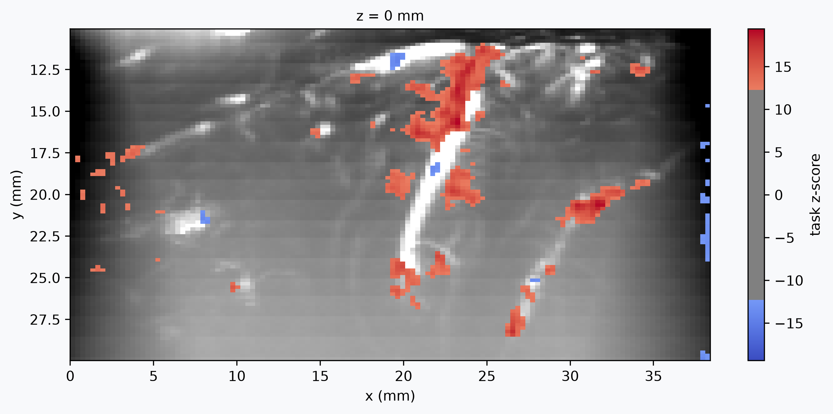
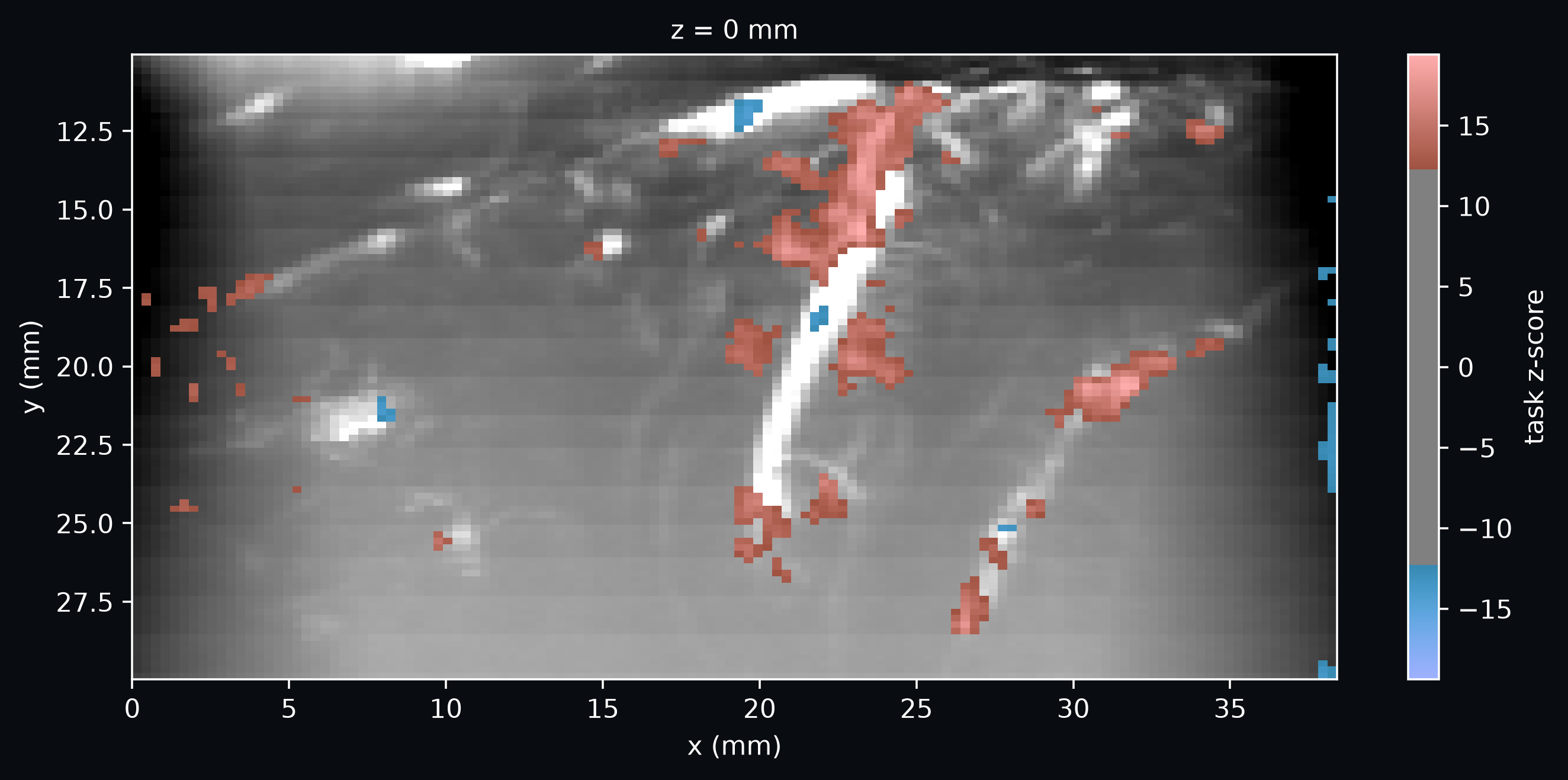
The z-map can be overlaid on the mean Doppler image with ConfUSIus's statistical map plotting helper. This is a lightweight reproduction of the Fig. 4D GLM map; here we threshold at the top 5% of positive task z-scores.
active_threshold = float(z_map.quantile(0.95))
active_voxels = z_map > active_threshold

plotter = z_map.fusi.plot.stat_map(
    bg_volume=mean_doppler,
    threshold=active_threshold,
    cmap=stat_cmap,
    cbar_label="task z-score",
    bg_color=bg_color,
)
Plot the strongest task-positive voxels
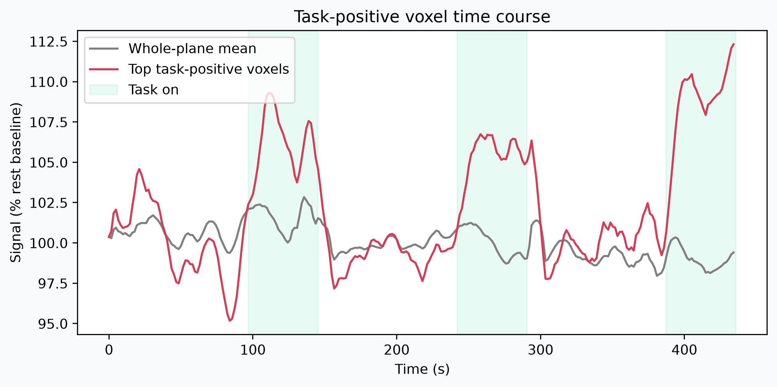
We average the Doppler traces from those task-positive voxels. This gives a quick sanity check that the voxels highlighted by the GLM follow the task blocks more clearly than the whole-plane average.
active_signal = scaled.where(active_voxels).mean(("z", "y", "x"))
mean_signal = scaled.mean(("z", "y", "x"))
fig, ax = plt.subplots(figsize=(9, 4), facecolor=bg_color)
mean_signal.plot(ax=ax, color="#808080", label="Whole-plane mean")
active_signal.plot(ax=ax, color="#d93a54", label="Top task-positive voxels")
for idx, event in enumerate(events.itertuples()):
    label = "Task on" if idx == 0 else None
    ax.axvspan(
        event.onset,
        event.onset + event.duration,
        color="#3ad9a4",
        alpha=0.12,
        label=label,
    )
ax.set_title("Task-positive voxel time course")
ax.set_xlabel("Time (s)")
ax.set_ylabel("Signal (% rest baseline)")

_ = ax.legend(loc="upper left")
Total running time: 54.8 s
Launch in Binder Download .py Download .ipynb
-
Rabut, Claire, et al. “Functional Ultrasound Imaging of Human Brain Activity through an Acoustically Transparent Cranial Window.” Science Translational Medicine, vol. 16, no. 749, May 2024, p. eadj3143. DOI.org (Crossref), https://doi.org/10.1126/scitranslmed.adj3143. ↩