Examples¶

These examples show how to use ConfUSIus on real data, with an emphasis on workflows you can run and adapt in your own analyses.

Each example starts from a plain Python script and is rendered as a notebook-style page with code, outputs, and downloadable source files.

Getting Started¶

First steps with ConfUSIus: loading a recording, working with Xarray-backed data, and building simple summaries and visualizations.

ConfUSIus and Xarray 101

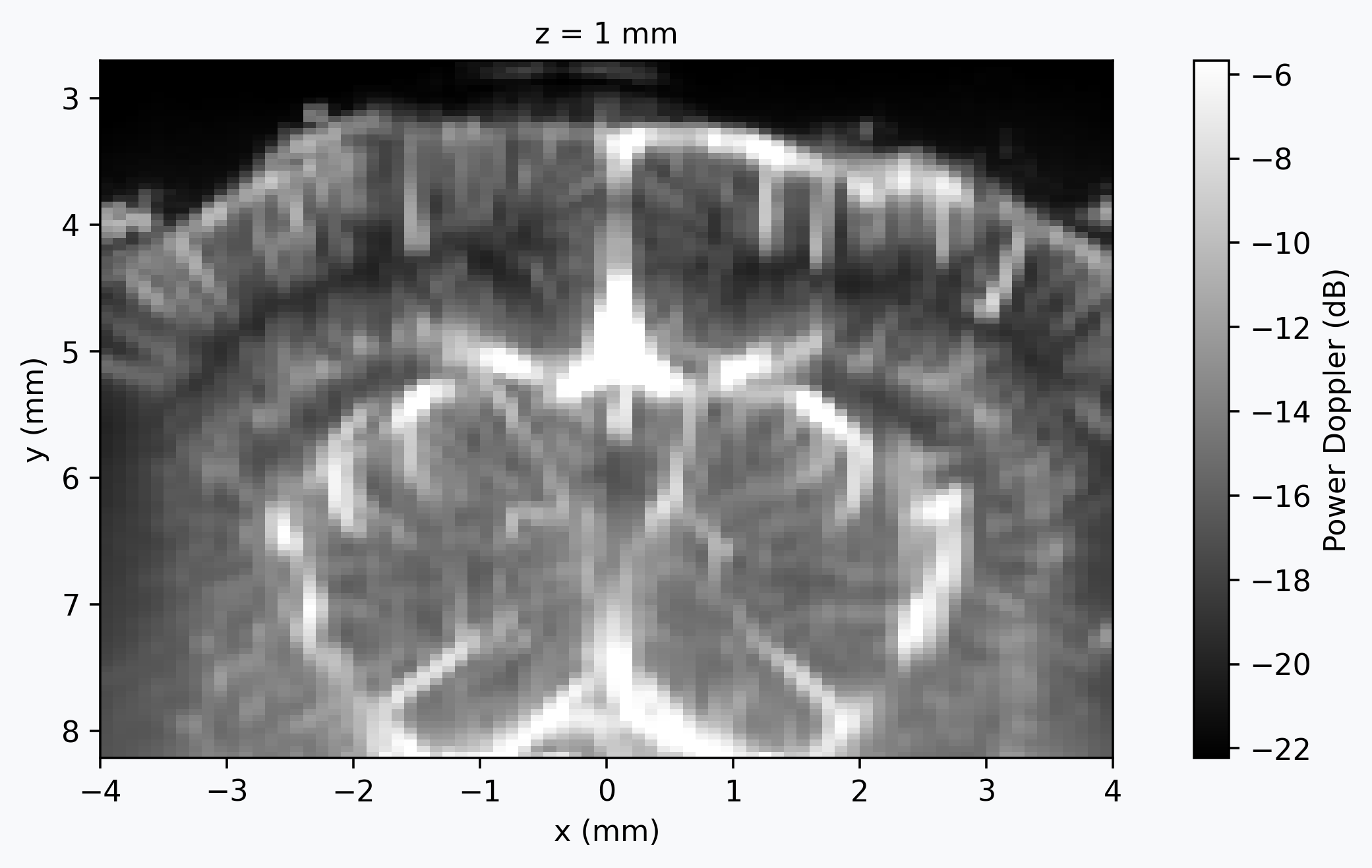
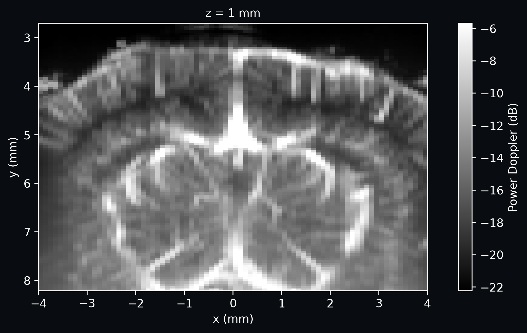
This example demonstrates how to use ConfUSIus to load and handle fUSI data as DataArray instances. We will use a small subset of the Nunez-Elizalde 2022 dataset and use a few basic Xarray operations to inspect, subset, and summarize the data.

Aligning fUSI recordings across sessions, subjects, or to a reference anatomy with ConfUSIus's volume registration tools.

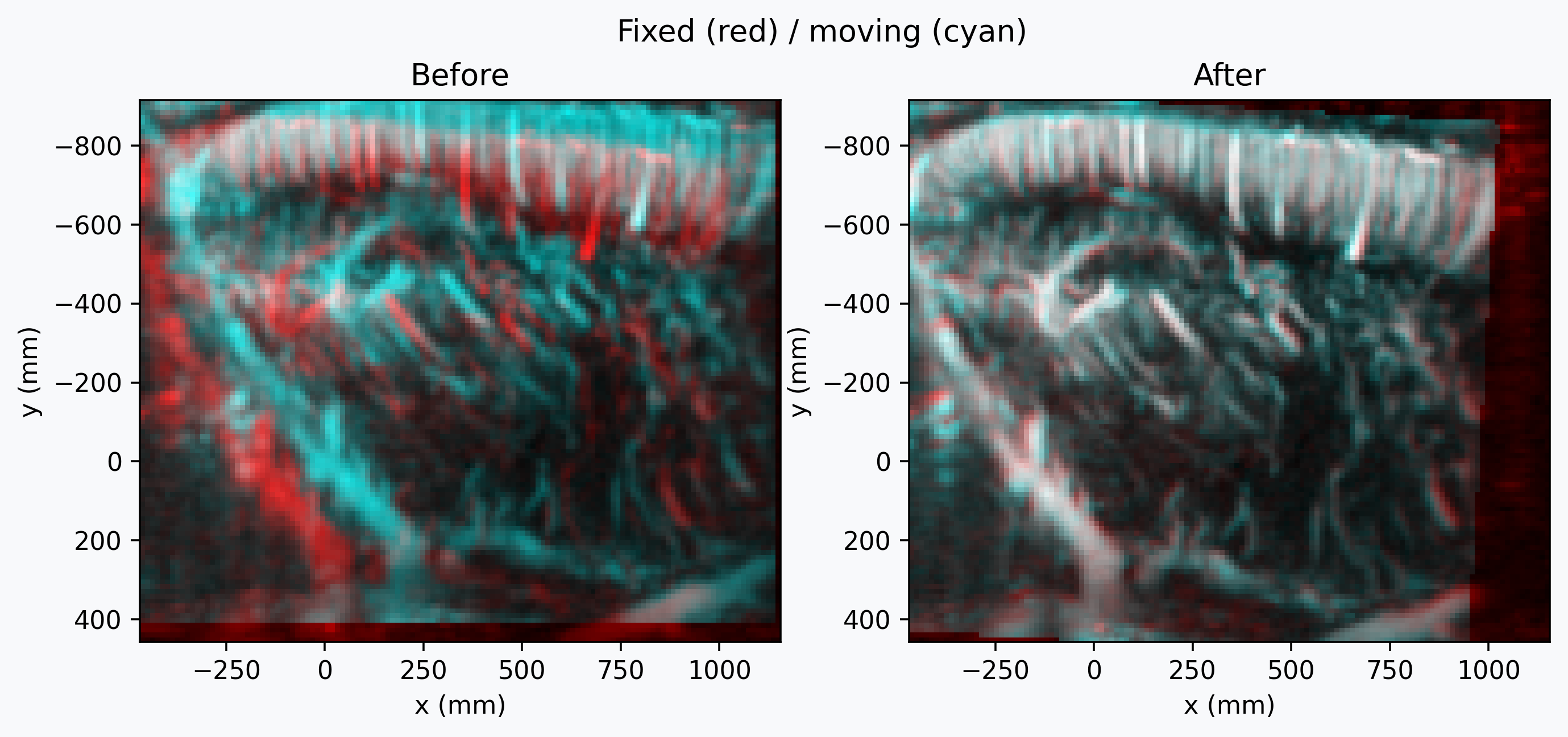
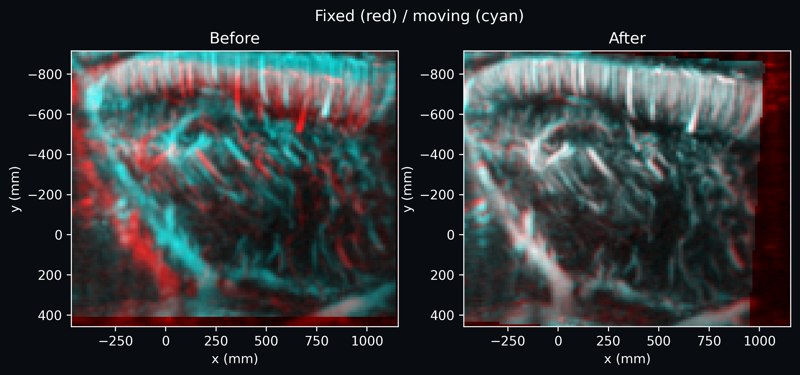
Registration of two sessions from the same subject

This example shows how to align two power Doppler images acquired from the same subject in different sessions. We use register_volume with a rigid transform, which is appropriate when the imaged anatomy is the same but the probe placement differs slightly between the two recordings.

Extracting spatiotemporal structure from fUSI recordings using dimensionality reduction techniques such as PCA, FastICA, and NMF.

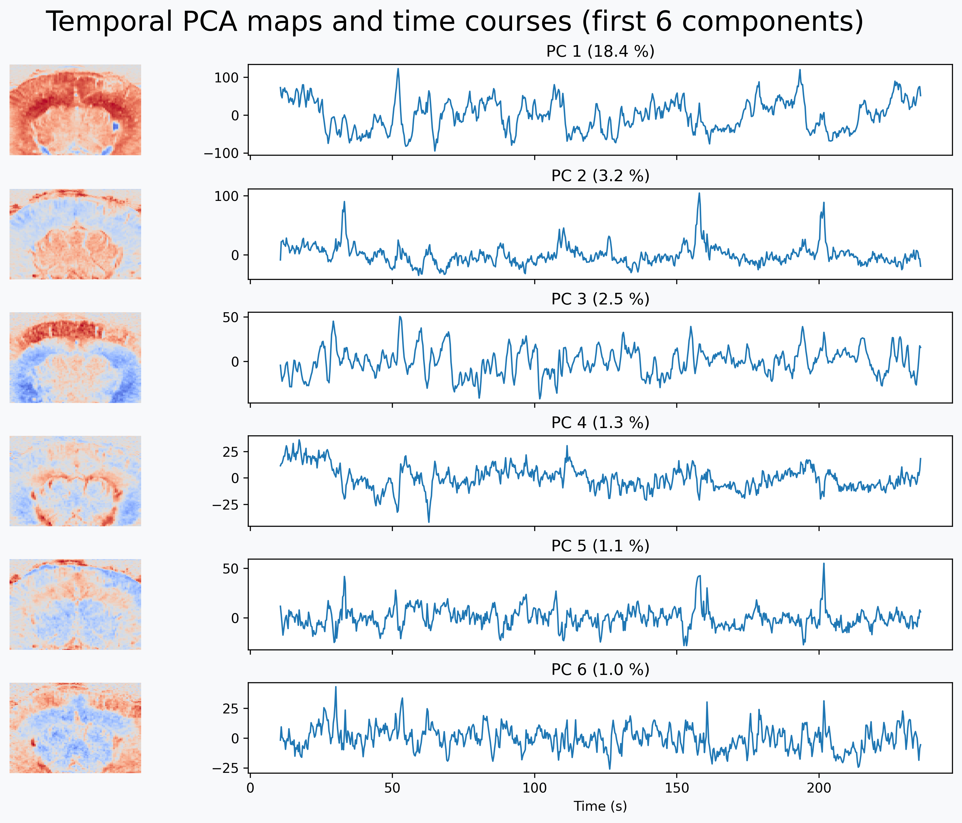
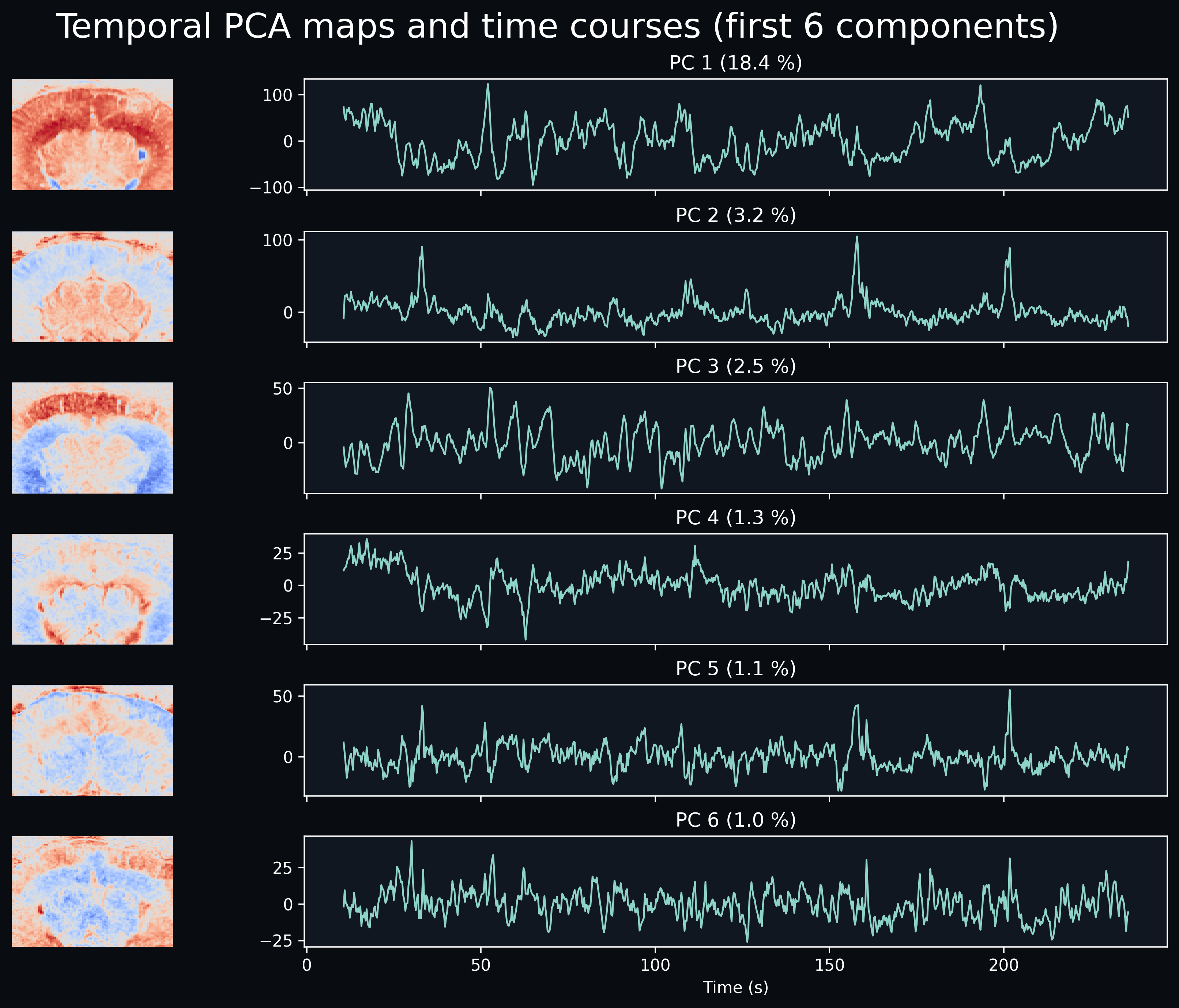
PCA on a single fUSI recording

This example shows how to use principal component analysis (PCA) to decompose a fUSI recording into principal axes of variance.
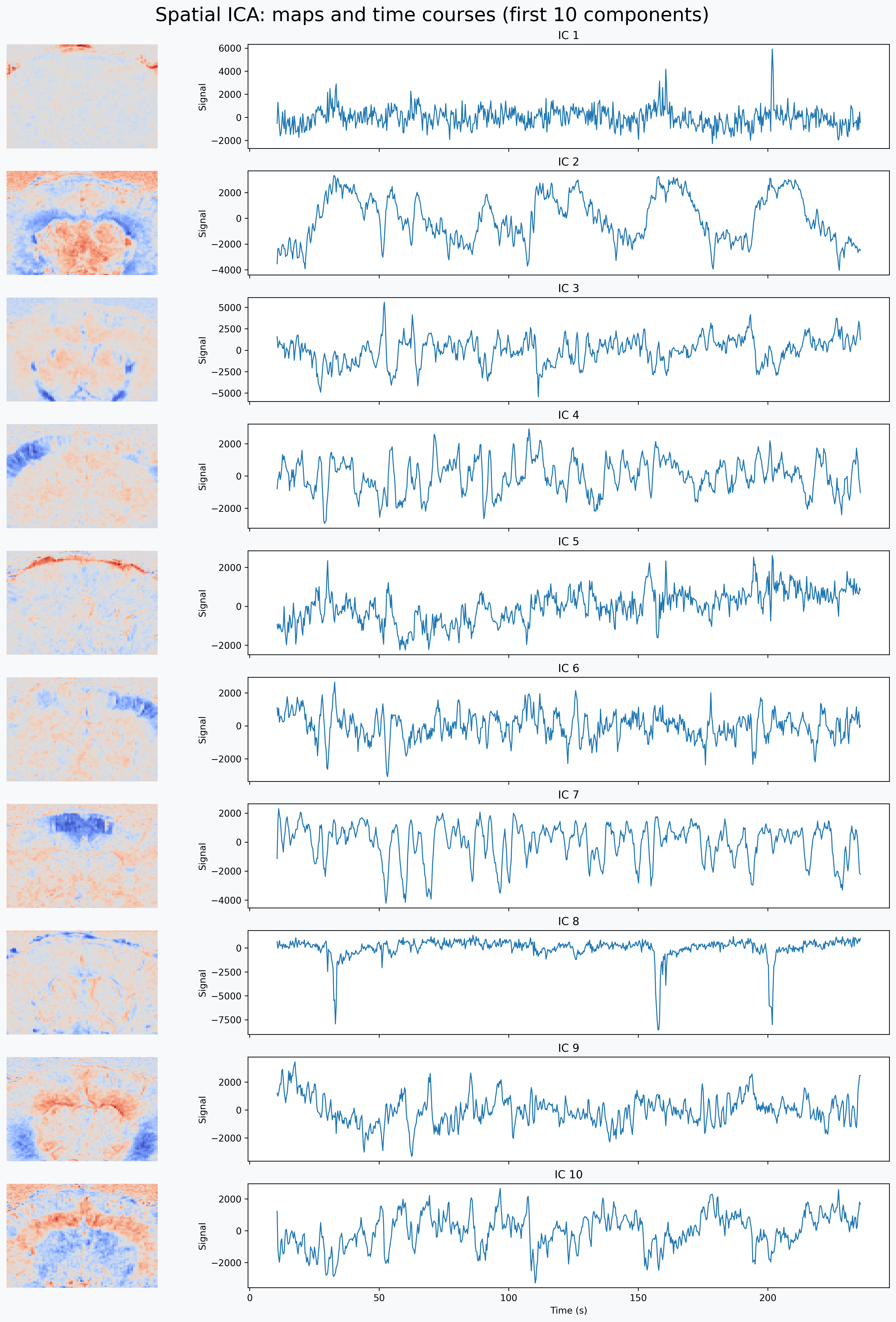
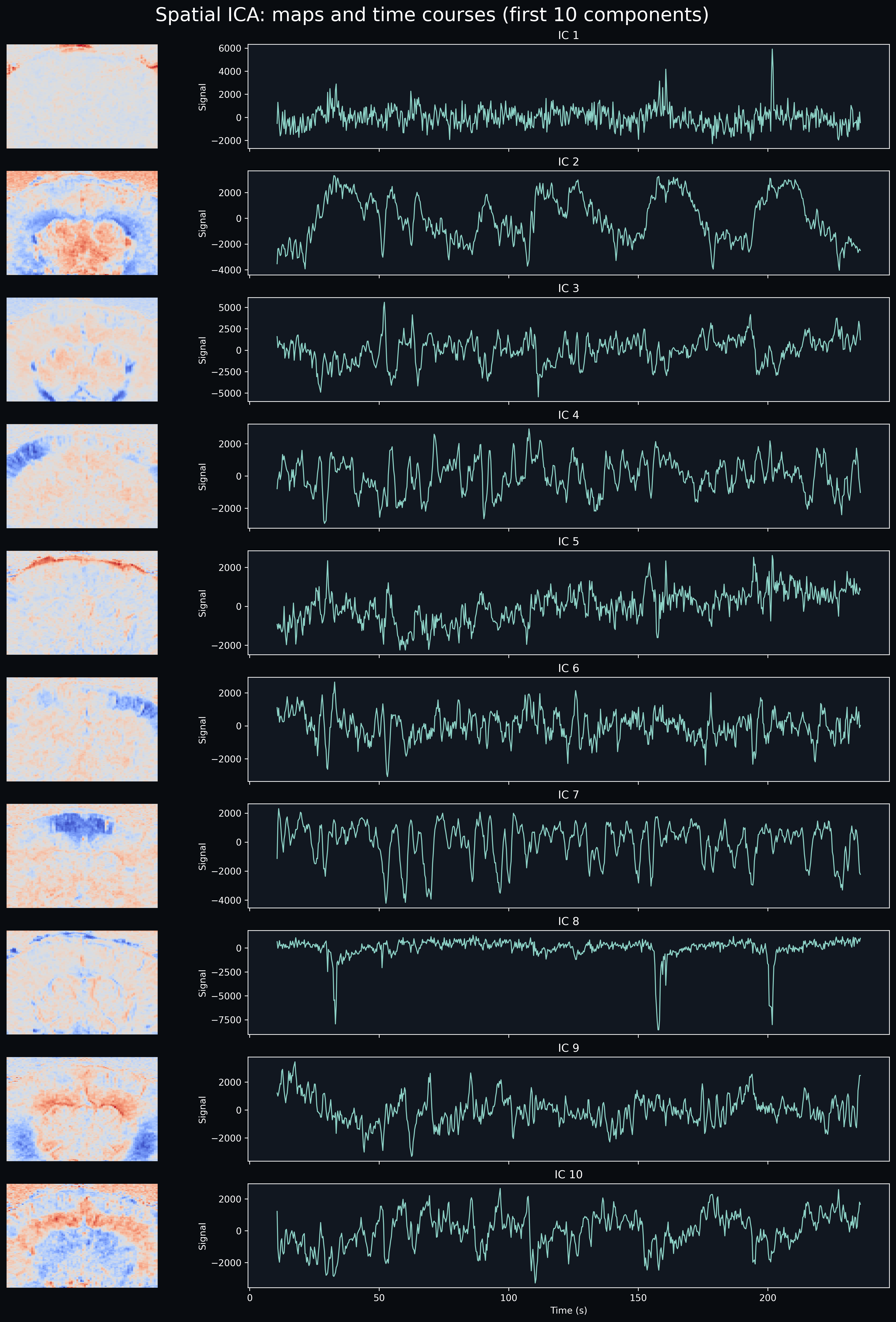
FastICA on a single fUSI recording

This example shows how to use FastICA to decompose a fUSI recording into independent components.
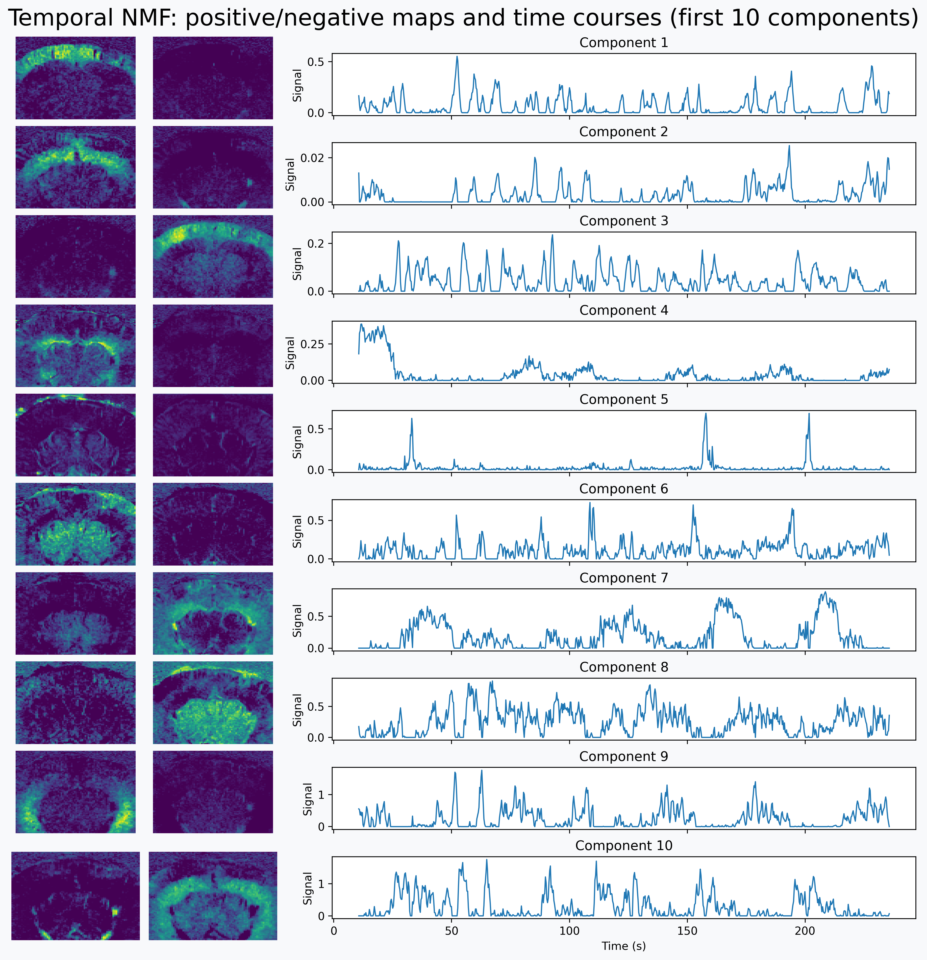
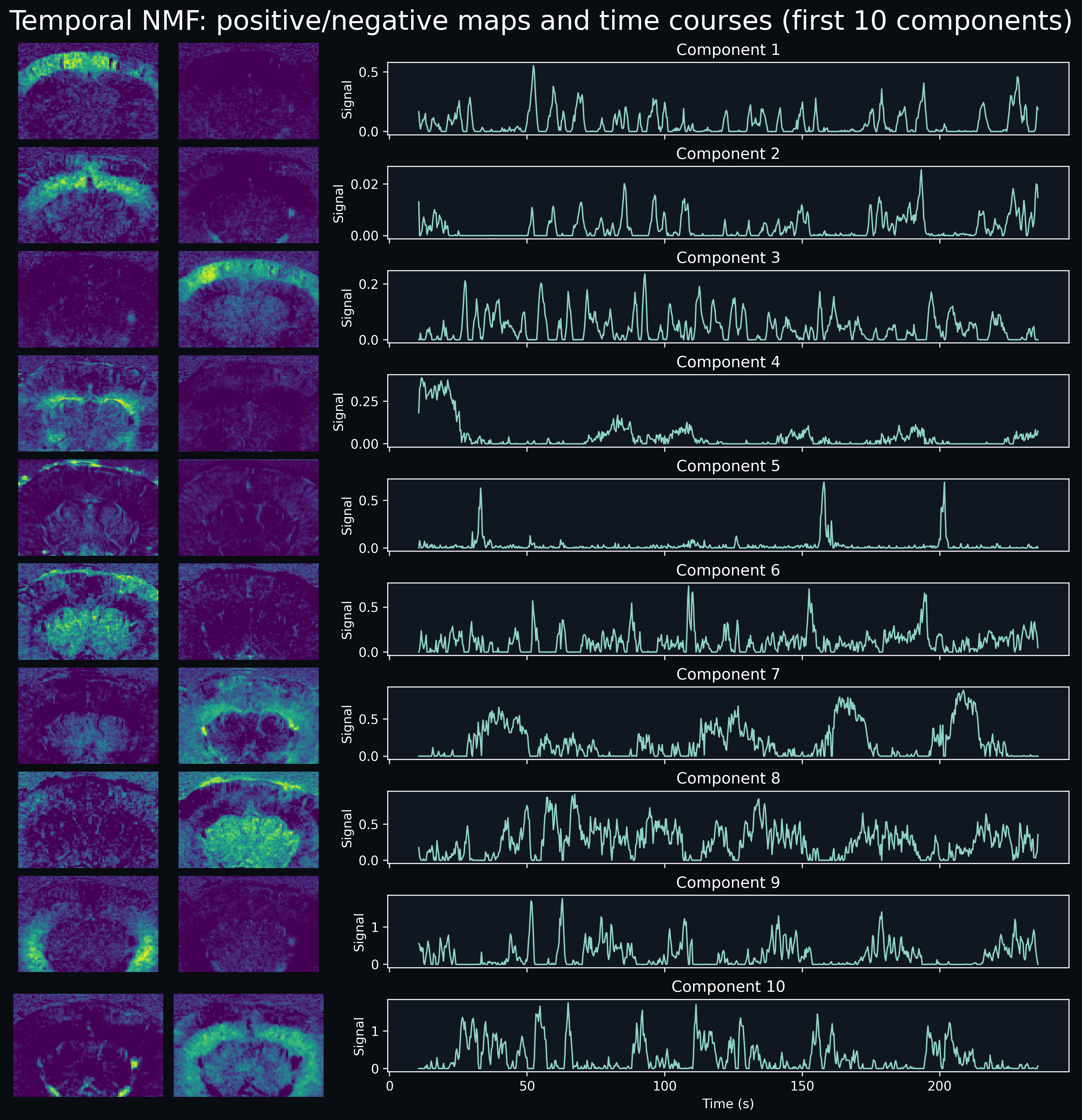
NMF on a single fUSI recording

This example shows how to use non-negative matrix factorization (NMF) to decompose a fUSI recording into non-negative spatial maps and their associated non-negative time courses. It complements the PCA and FastICA examples in the same gallery.

Computing functional connectivity (FC) measures from fUSI data using brain region parcellations or data-driven approaches.

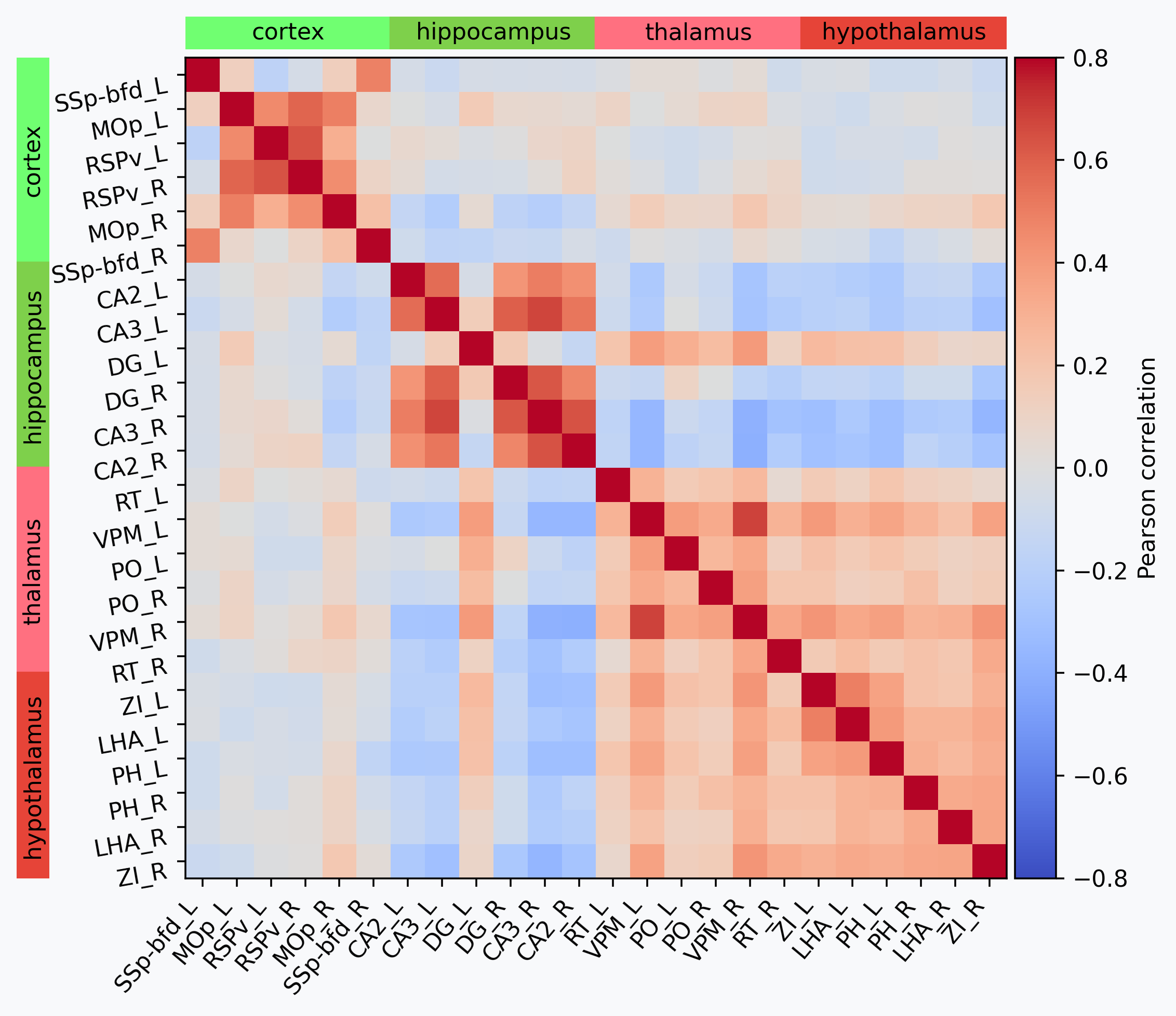
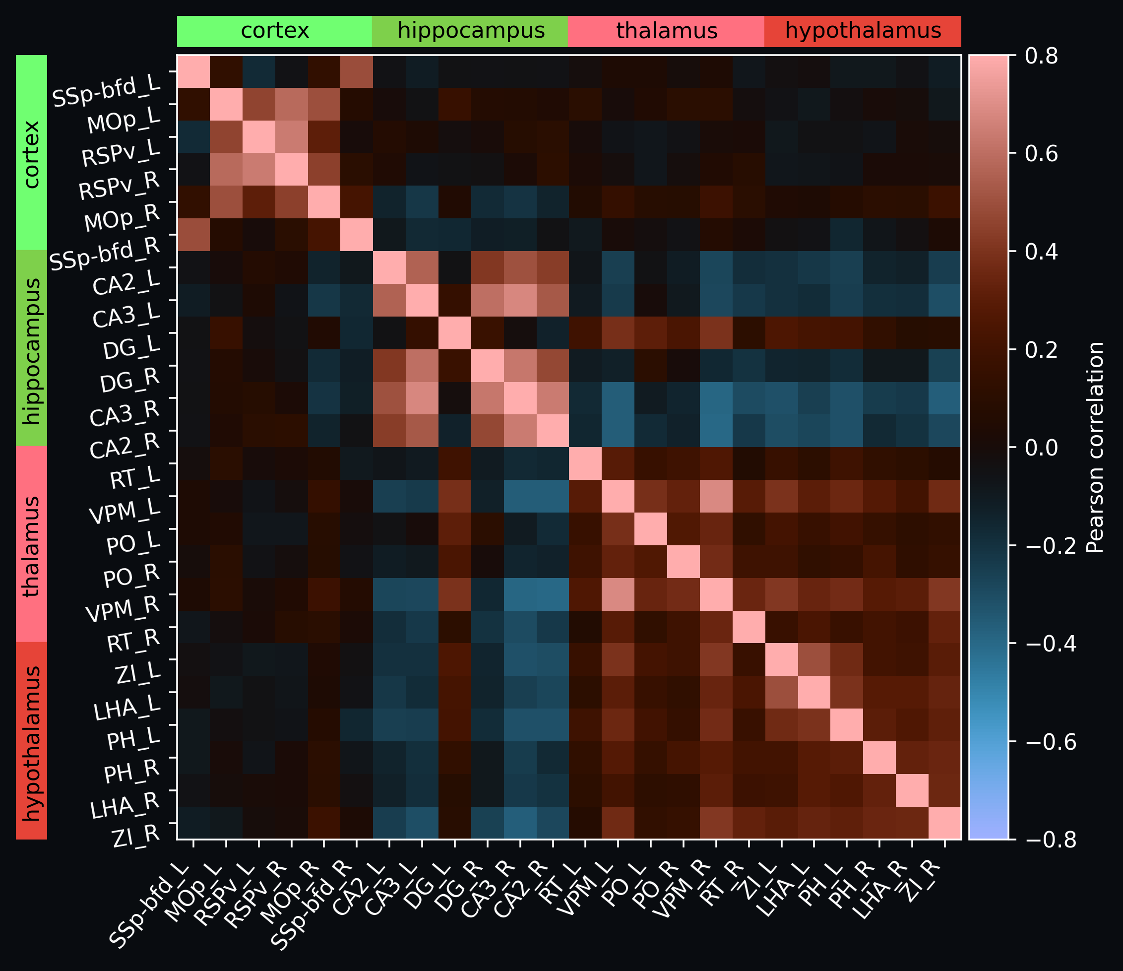
Atlas-based region correlation matrix

This example shows an end-to-end regional functional connectivity (FC) analysis: register a single-slice fUSI recording to an Allen-space template, bring the Allen Mouse Brain Atlas into the recording's native space, extract region-averaged signals, and visualise their pairwise correlation with plot_matrix.
Atlas-based seed connectivity maps

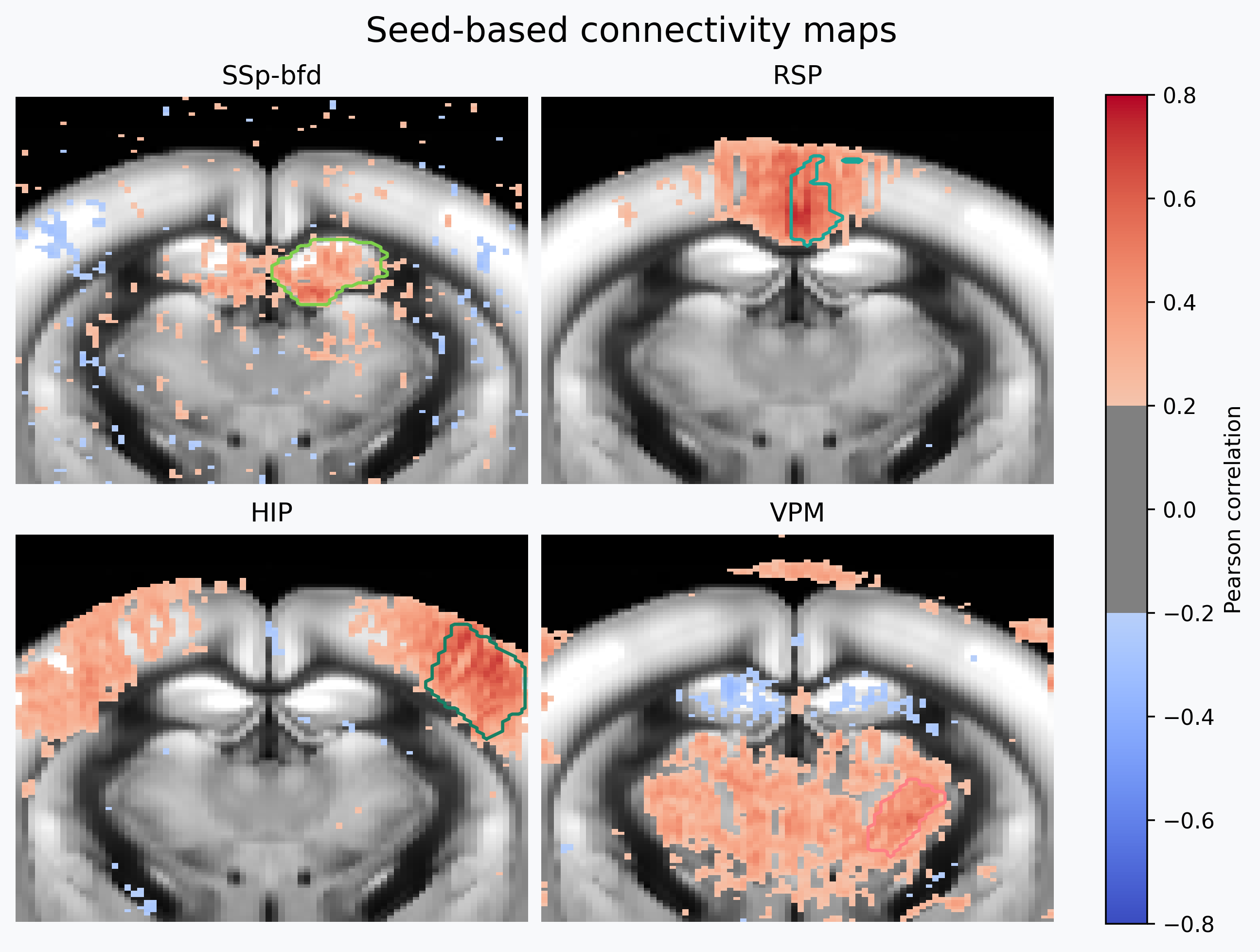
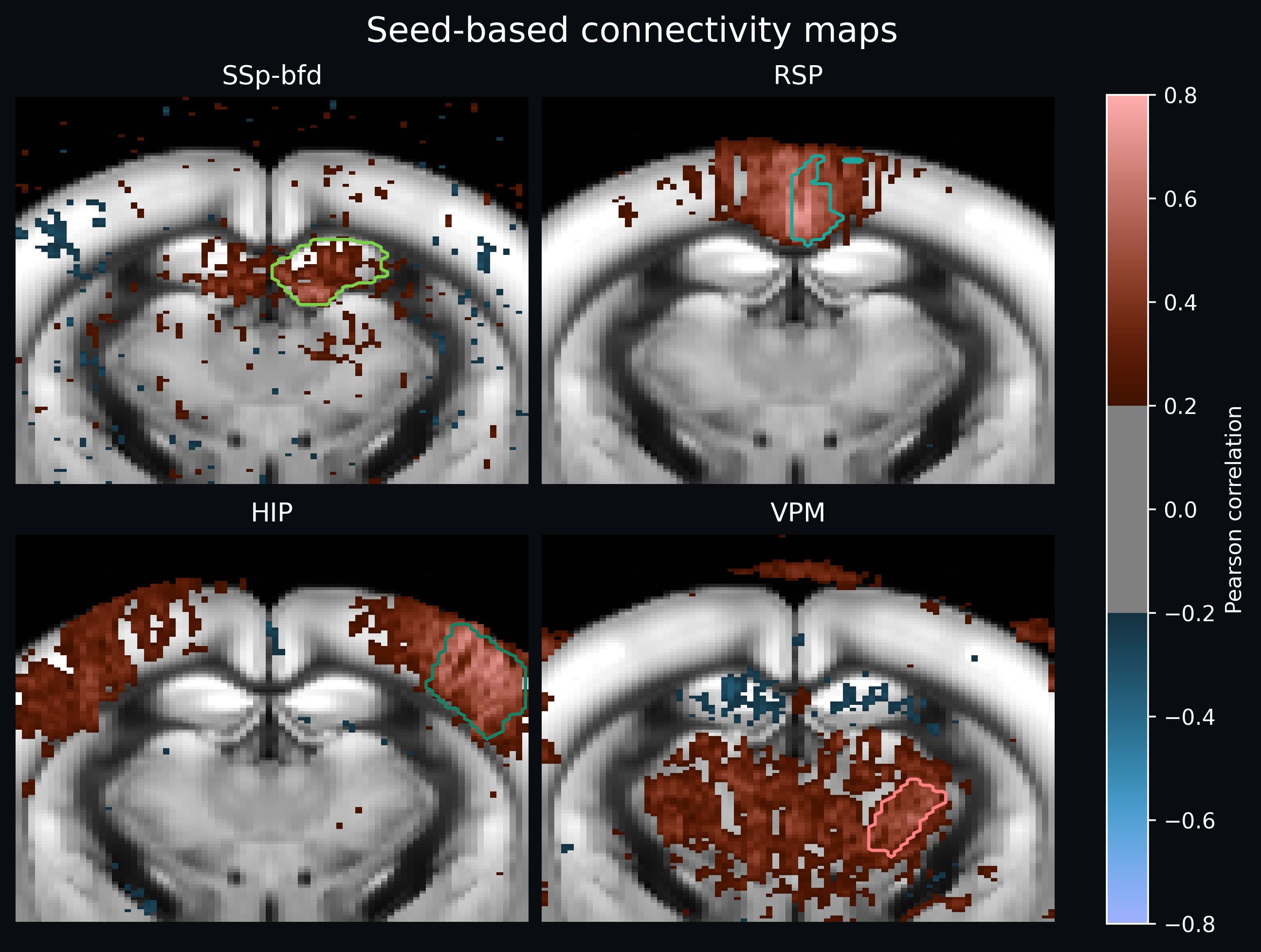
This example computes voxel-wise seed-based functional connectivity maps: register a single-slice fUSI recording to an Allen-space template, bring an Allen Mouse Brain Atlas into the recording's native space, pick four atlas regions of interest as seeds, and correlate each seed's signal against every voxel with SeedBasedMaps. Each resulting map is displayed with plot_stat_map, using the resampled Allen reference volume as background.