Atlas correlation matrix
Atlas-based region correlation matrix
This example shows an end-to-end regional functional connectivity (FC) analysis:
register a single-slice fUSI recording to an Allen-space template, bring the plot_matrix.
We use an awake freely-running acquisition from subject CR022, session 20201007,
in the Nunez-Elizalde 2022 dataset,
and the
Fetch the recording and the template
The recording is a single coronal slice imaged for approximately 4 minutes at 3.33 Hz. Registration works on a static anatomical image, so we use the temporal mean, converted to decibels for a more stable dynamic range.
from pathlib import Path

import matplotlib as mpl
import matplotlib.pyplot as plt
import numpy as np
import xarray as xr

import confusius as cf

# Adapt background color to the current Matplotlib style.
bg_color = mpl.colors.to_hex(mpl.rcParams["figure.facecolor"])

xr.set_options(display_expand_data=False)

template = cf.datasets.fetch_template_pepe_mariani_2026()

bids_root = cf.datasets.fetch_nunez_elizalde_2022(
    subjects="CR022", sessions="20201007", tasks="spontaneous", acqs="slice02"
)

data_path = (
    Path(bids_root)
    / "sub-CR022"
    / "ses-20201007"
    / "fusi"
    / "sub-CR022_ses-20201007_task-spontaneous_acq-slice02_pwd.nii.gz"
)
# The recording's timepoints are not perfectly uniformly spaced so we resample to a
# uniform grid before any time-domain processing (filtering below requires it).
data = cf.timing.resample_to_uniform_time(cf.load(data_path))
moving = data.mean(dim="time").fusi.scale.db().compute()

data
/tmp/ipykernel_13546/685735078.py:30: UserWarning: Time coordinate is non-uniform; using the median step to build a uniform target grid.
  data = cf.timing.resample_to_uniform_time(cf.load(data_path))
- time: 755
- z: 1
- y: 125
- x: 80
- dask.array<chunksize=(755, 1, 125, 80), meta=np.ndarray>
Array Chunk Bytes 57.60 MiB 57.60 MiB Shape (755, 1, 125, 80) (755, 1, 125, 80) Dask graph 1 chunks in 7 graph layers Data type float64 numpy.ndarray - time(time)float6411.0 11.3 11.6 ... 236.9 237.2
- units :
- s
- volume_acquisition_reference :
- start
- volume_acquisition_duration :
- 0.3
array([ 10.998, 11.298, 11.598, ..., 236.598, 236.898, 237.198], shape=(755,))
- z(z)float640.4
- units :
- mm
- voxdim :
- 0.4000000059604645
array([0.4])
- y(y)float642.996 3.044 3.092 ... 8.939 8.988
- units :
- mm
- voxdim :
- 0.04831999912858009
array([2.99584, 3.04416, 3.09248, 3.1408 , 3.18912, 3.23744, 3.28576, 3.33408, 3.3824 , 3.43072, 3.47904, 3.52736, 3.57568, 3.624 , 3.67232, 3.72064, 3.76896, 3.81728, 3.8656 , 3.91392, 3.96224, 4.01056, 4.05888, 4.1072 , 4.15552, 4.20384, 4.25216, 4.30048, 4.3488 , 4.39712, 4.44544, 4.49376, 4.54208, 4.5904 , 4.63872, 4.68704, 4.73536, 4.78368, 4.832 , 4.88032, 4.92864, 4.97696, 5.02528, 5.0736 , 5.12192, 5.17024, 5.21856, 5.26688, 5.3152 , 5.36352, 5.41184, 5.46016, 5.50848, 5.5568 , 5.60512, 5.65344, 5.70176, 5.75008, 5.7984 , 5.84672, 5.89504, 5.94336, 5.99168, 6.04 , 6.08832, 6.13664, 6.18496, 6.23328, 6.2816 , 6.32992, 6.37824, 6.42656, 6.47488, 6.5232 , 6.57152, 6.61984, 6.66816, 6.71648, 6.7648 , 6.81312, 6.86144, 6.90976, 6.95808, 7.0064 , 7.05472, 7.10304, 7.15136, 7.19968, 7.248 , 7.29632, 7.34464, 7.39296, 7.44128, 7.4896 , 7.53792, 7.58624, 7.63456, 7.68288, 7.7312 , 7.77952, 7.82784, 7.87616, 7.92448, 7.9728 , 8.02112, 8.06944, 8.11776, 8.16608, 8.2144 , 8.26272, 8.31104, 8.35936, 8.40768, 8.456 , 8.50432, 8.55264, 8.60096, 8.64928, 8.6976 , 8.74592, 8.79424, 8.84256, 8.89088, 8.9392 , 8.98752]) - x(x)float64-3.95 -3.85 -3.75 ... 3.85 3.95
- units :
- mm
- voxdim :
- 0.10000000149011612
array([-3.95, -3.85, -3.75, -3.65, -3.55, -3.45, -3.35, -3.25, -3.15, -3.05,
       -2.95, -2.85, -2.75, -2.65, -2.55, -2.45, -2.35, -2.25, -2.15, -2.05,
       -1.95, -1.85, -1.75, -1.65, -1.55, -1.45, -1.35, -1.25, -1.15, -1.05,
       -0.95, -0.85, -0.75, -0.65, -0.55, -0.45, -0.35, -0.25, -0.15, -0.05,
        0.05,  0.15,  0.25,  0.35,  0.45,  0.55,  0.65,  0.75,  0.85,  0.95,
        1.05,  1.15,  1.25,  1.35,  1.45,  1.55,  1.65,  1.75,  1.85,  1.95,
        2.05,  2.15,  2.25,  2.35,  2.45,  2.55,  2.65,  2.75,  2.85,  2.95,
        3.05,  3.15,  3.25,  3.35,  3.45,  3.55,  3.65,  3.75,  3.85,  3.95])
- qform_code :
- 1
- manufacturer :
- Verasonics
- manufacturers_model_name :
- Vantage 128
- software_version :
- Alan Urban Technology & Consulting (AUTC)
- probe_manufacturer :
- Vermon
- probe_type :
- linear
- probe_model :
- L22-XTech
- probe_central_frequency :
- 15000000.0
- probe_number_of_elements :
- 128
- probe_pitch :
- 0.1
- probe_focal_width :
- 0.4
- probe_focal_depth :
- 8.0
- power_doppler_integration_duration :
- 0.3
- power_doppler_integration_stride :
- 0.3
- clutter_filter_window_duration :
- 0.4
- clutter_filter_window_stride :
- 0.3
- clutter_filters :
- ['highpass:15Hz', 'svd:remove_first_15_components']
- task_name :
- spontaneous
- task_description :
- Spontaneous activity without explicit visual stimulation.
- depth :
- [0.0, 5.991680000000001]
- transmit_frequency :
- 15625000.0
- compound_sampling_frequency :
- 500.0
- plane_wave_angles :
- [-10.0, -7.9, -5.8, -3.6999999999999993, -1.5999999999999996, 0.5000000000000018, 2.6000000000000014, 4.700000000000002, 6.8000000000000025, 8.900000000000002]
- probe_voltage :
- 25.0
- affines :
- {'physical_to_qform': array([[1., 0., 0., 0.], [0., 1., 0., 0.], [0., 0., 1., 0.], [0., 0., 0., 1.]])}
Register the recording to the template
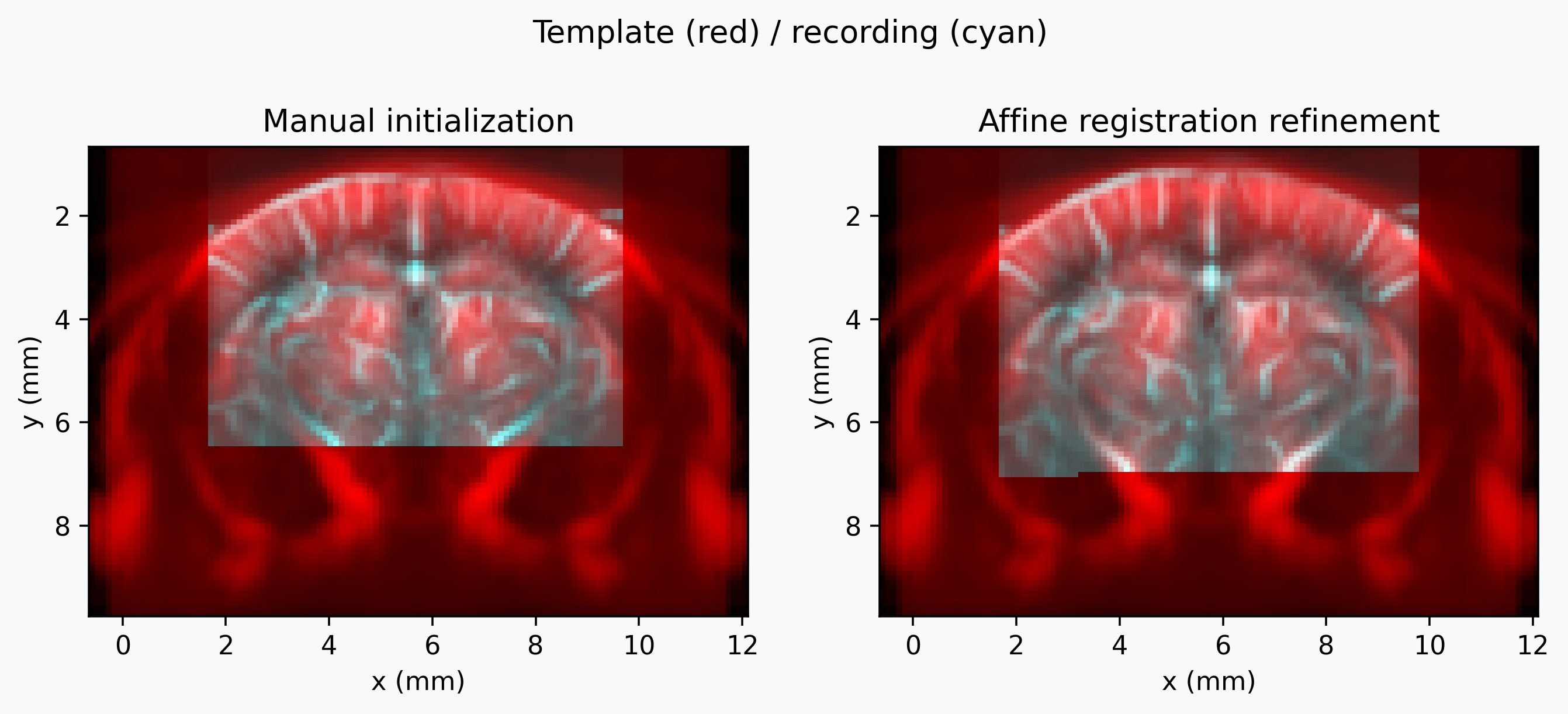
The template is a 3D volume but the recording is a single slice. We can still register the recording to the template, but we need to initialize the registration with a rough guess of where the recording sits in the template, otherwise the registration algorithm may not converge to the right slice. To initialize the registration, we use an affine transform obtained using napari's manual transform tool by placing the recording at an approximate location on the template. The transform is not perfect, but it is close enough to allow the registration algorithm to converge to a good solution.
register_volume expects a transform
mapping fixed (template) physical coordinates to moving (recording) physical
coordinates, so we invert the Napari affine—which instead describes how to place the
recording into the template's coordinate system—before using it as initialization.
napari_affine = np.array(
    [
        [1.0, 0.0, 0.0, 5.594638656430411],
        [0.0, 1.0, 0.0, -2.50293925701927],
        [0.0, 0.0, 1.0, 5.6650243788545875],
        [0.0, 0.0, 0.0, 1.0],
    ]
)
initialization = np.linalg.inv(napari_affine)

# Crop the template to a thin band around the recording's expected location to improve
# registration speed and visualization.
target_z = napari_affine[0, 3] + float(moving.z.values[0])
fixed = template.sel(z=slice(target_z - 1.0, target_z + 1.0)).fusi.scale.db()

initialized = cf.registration.resample_like(
    moving, fixed, initialization, default_value=float(moving.min())
)
_ = cf.plotting.plot_composite(
    fixed,
    initialized,
    slice_coords=[target_z],
    normalize_strategy="per_slice",
    bg_color=bg_color,
)
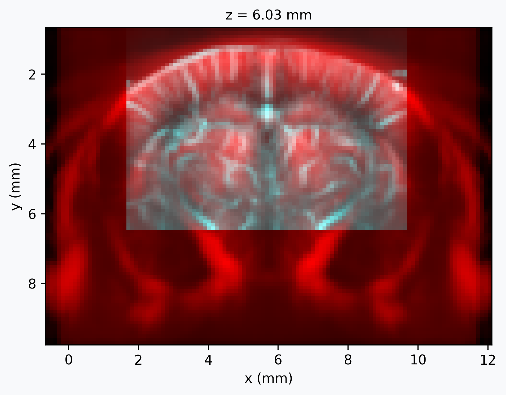
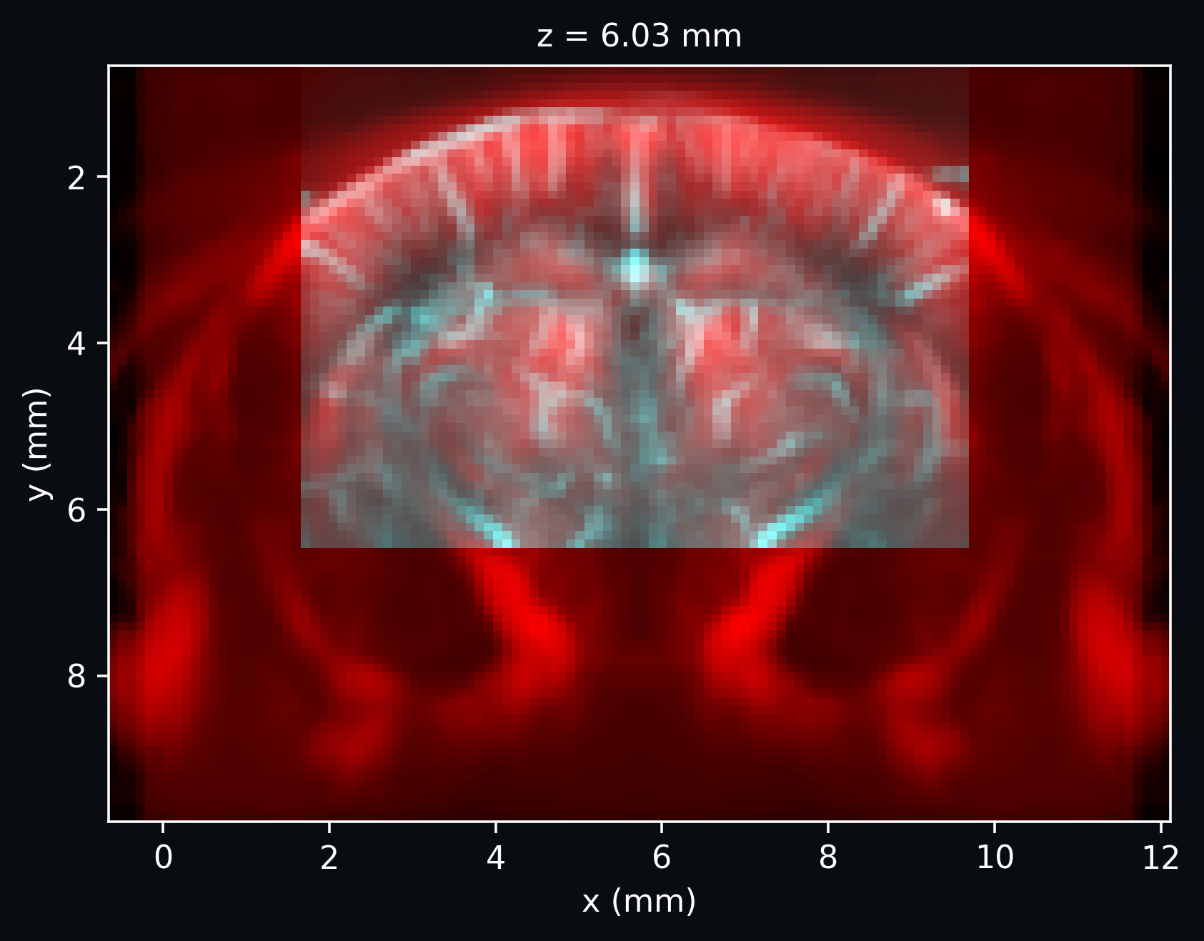
We use an affine transform: on top of the rotation and translation a rigid transform would allow, it also captures small scale and shear differences between the recording and the template.
registered, affine, _ = cf.registration.register_volume(
    moving=moving,
    fixed=fixed,
    transform_type="affine",
    metric="correlation",
    convergence_window_size=50,
    number_of_iterations=500,
    learning_rate=1,
    initialization=initialization,
    show_progress=True,
)
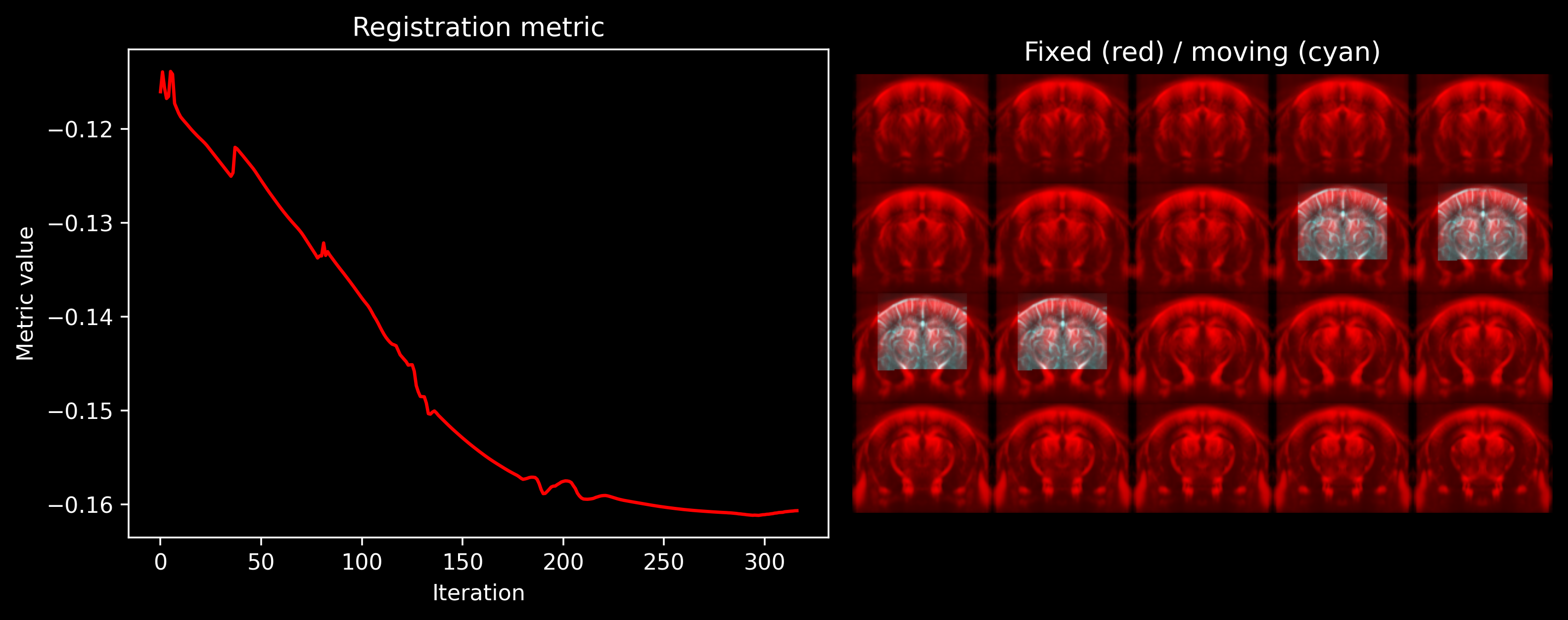
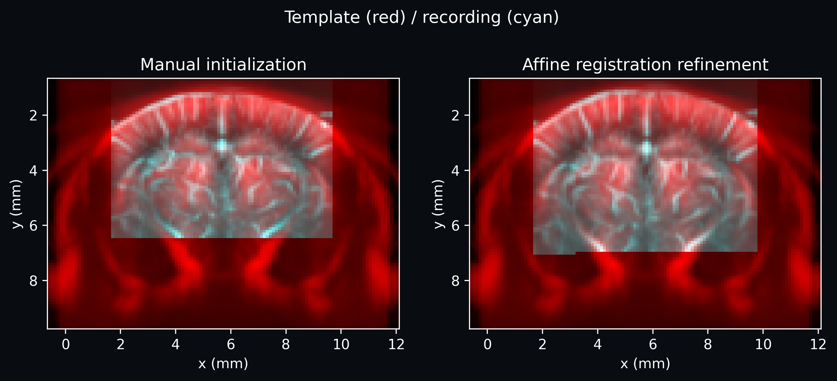
The initialization was already close, so the refinement is small. Comparing the overlay before and after registration, alignment is slightly better after the affine refinement, most noticeably around the anterior choroidal arteries in the bottom part of the field of view.
fig, axes = plt.subplots(1, 2, figsize=(10, 4))
fig.patch.set_facecolor(bg_color)
for ax, moving_view, title in [
    (axes[0], initialized, "Manual initialization"),
    (axes[1], registered, "Affine registration refinement"),
]:
    cf.plotting.plot_composite(
        fixed,
        moving_view,
        axes=ax,
        slice_coords=[target_z],
        normalize_strategy="per_slice",
        bg_color=bg_color,
    )
    ax.set_title(title)

_ = fig.suptitle("Template (red) / recording (cyan)")
Resample the Allen atlas onto the recording's native grid
The template is not itself expressed in Allen space, but it carries the affine
transform to get there in template.attrs["affines"]["physical_to_sform"]. Composing
it with the inverse of the estimated registration affine gives a single transform from
the recording's native coordinates directly to Allen atlas coordinates.
physical_to_sform = template.attrs["affines"]["physical_to_sform"]
subject_to_atlas = physical_to_sform @ np.linalg.inv(affine)

atlas = cf.atlas.Atlas.from_brainglobe("allen_mouse_100um")
atlas_native = atlas.resample_like(moving, subject_to_atlas)

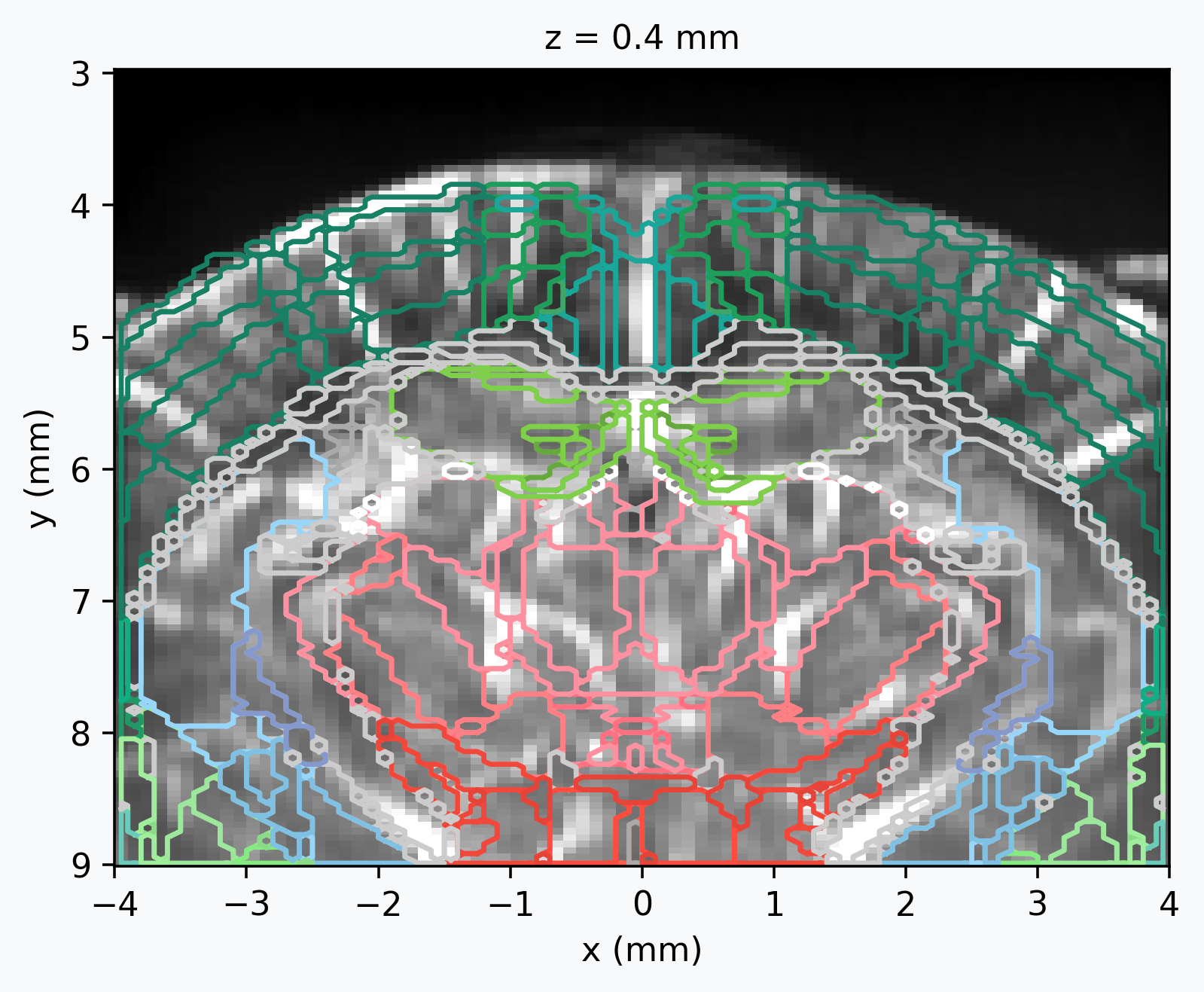
plotter = cf.plotting.plot_volume(
    moving, slice_mode="z", cmap="gray", show_colorbar=False, bg_color=bg_color
)
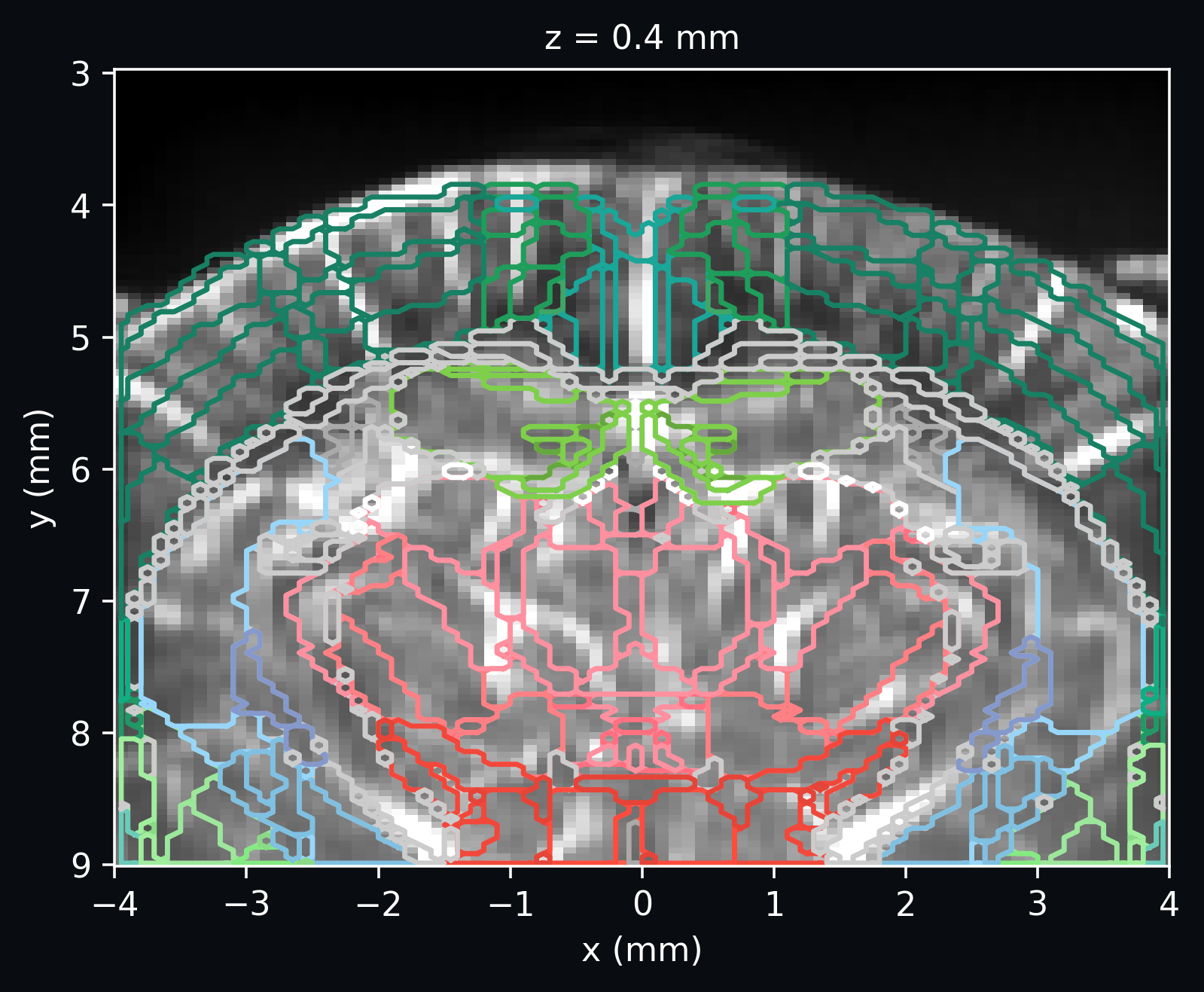
_ = plotter.add_contours(atlas_native.annotation)
Extract region signals and compute their correlation matrix
Atlas.get_masks accepts parent acronyms from the
Allen ontology (e.g. "SSp-bfd") and automatically aggregates every descendant
region, so we can request a handful of coarse regions per area of interest instead of
individual cortical layers or thalamic nuclei. We pick three regions each from cortex,
hippocampus, thalamus, and hypothalamus.
We extract left and right hemispheres separately via
get_masks's sides argument: combining both
sides into one mask would average left/right signals together and hide
bilateral FC and interhemispheric differences.
get_masks reuses the same region id for both
hemispheres of a region, so we stack the two sides' masks into a single (mask, z, y,
x) array and give every layer a unique id before passing it to
extract_with_labels in one call. Within
each area the left hemisphere is ordered lateral-to-medial and the right
medial-to-lateral, so each area block reads as one continuous sweep across the slice.
groups = {
    "cortex": ["RSPv", "MOp", "SSp-bfd"],
    "hippocampus": ["DG", "CA3", "CA2"],
    "thalamus": ["PO", "VPM", "RT"],
    "hypothalamus": ["PH", "LHA", "ZI"],
}
# Allen CCF ids for each area's parent division, used below to color the group strips
# with the atlas's own official colors instead of arbitrary ones.
division_ids = {"cortex": 315, "hippocampus": 1089, "thalamus": 549, "hypothalamus": 1097}
group_colors = {
    area: "#{:02x}{:02x}{:02x}".format(*atlas.lookup.loc[division_id, "rgb_triplet"])
    for area, division_id in division_ids.items()
}
region_acronyms = [acronym for acronyms in groups.values() for acronym in acronyms]

region_order = []
group_labels = []
for area, acronyms in groups.items():
    region_order += [f"{acronym}_L" for acronym in reversed(acronyms)]
    region_order += [f"{acronym}_R" for acronym in acronyms]
    group_labels += [area] * (2 * len(acronyms))

sides = ["left"] * len(region_acronyms) + ["right"] * len(region_acronyms)
mask_names = [f"{acronym}_L" for acronym in region_acronyms] + [
    f"{acronym}_R" for acronym in region_acronyms
]
masks = atlas_native.get_masks(region_acronyms * 2, sides=sides).assign_coords(
    mask=mask_names
)
# get_masks reuses the same region id for both hemispheres of a region, which
# extract_with_labels would reject as a duplicate id across stacked-mask layers. Give
# every layer a unique nonzero id instead; extract_with_labels names each output
# region from the mask coordinate above, not from these ids.
layer_ids = xr.DataArray(np.arange(1, masks.sizes["mask"] + 1), dims="mask")
masks = xr.where(masks != 0, layer_ids, 0)

signals = cf.extract.extract_with_labels(data, masks, reduction="mean")
# extract_with_labels does not guarantee any particular region order, so reindex
# explicitly into the left-right sweep computed above.
signals = signals.sel(region=region_order)

signals
- time: 755
- region: 24
- dask.array<chunksize=(755, 24), meta=np.ndarray>
Array Chunk Bytes 141.56 kiB 141.56 kiB Shape (755, 24) (755, 24) Dask graph 1 chunks in 13 graph layers Data type float64 numpy.ndarray - time(time)float6411.0 11.3 11.6 ... 236.9 237.2
- units :
- s
- volume_acquisition_reference :
- start
- volume_acquisition_duration :
- 0.3
array([ 10.998, 11.298, 11.598, ..., 236.598, 236.898, 237.198], shape=(755,))
- region(region)<U9'SSp-bfd_L' 'MOp_L' ... 'ZI_R'
array(['SSp-bfd_L', 'MOp_L', 'RSPv_L', 'RSPv_R', 'MOp_R', 'SSp-bfd_R', 'CA2_L',
       'CA3_L', 'DG_L', 'DG_R', 'CA3_R', 'CA2_R', 'RT_L', 'VPM_L', 'PO_L',
       'PO_R', 'VPM_R', 'RT_R', 'ZI_L', 'LHA_L', 'PH_L', 'PH_R', 'LHA_R',
       'ZI_R'], dtype='<U9')
- qform_code :
- 1
- manufacturer :
- Verasonics
- manufacturers_model_name :
- Vantage 128
- software_version :
- Alan Urban Technology & Consulting (AUTC)
- probe_manufacturer :
- Vermon
- probe_type :
- linear
- probe_model :
- L22-XTech
- probe_central_frequency :
- 15000000.0
- probe_number_of_elements :
- 128
- probe_pitch :
- 0.1
- probe_focal_width :
- 0.4
- probe_focal_depth :
- 8.0
- power_doppler_integration_duration :
- 0.3
- power_doppler_integration_stride :
- 0.3
- clutter_filter_window_duration :
- 0.4
- clutter_filter_window_stride :
- 0.3
- clutter_filters :
- ['highpass:15Hz', 'svd:remove_first_15_components']
- task_name :
- spontaneous
- task_description :
- Spontaneous activity without explicit visual stimulation.
- depth :
- [0.0, 5.991680000000001]
- transmit_frequency :
- 15625000.0
- compound_sampling_frequency :
- 500.0
- plane_wave_angles :
- [-10.0, -7.9, -5.8, -3.6999999999999993, -1.5999999999999996, 0.5000000000000018, 2.6000000000000014, 4.700000000000002, 6.8000000000000025, 8.900000000000002]
- probe_voltage :
- 25.0
- affines :
- {'physical_to_qform': array([[1., 0., 0., 0.], [0., 1., 0., 0.], [0., 0., 1., 0.], [0., 0., 0., 1.]])}
Clean the region signals
Before correlating regions we remove nuisance variance that would otherwise inflate
their apparent FC: a 0.01 Hz high-pass filter for slow drift, and one
aCompCor component regressed out.
aCompCor components are extracted from white matter voxels—the Allen ontology's
"fiber tracts" division—so they must be computed from the voxelwise recording rather
than the already-averaged regions.
white_matter = atlas_native.get_masks("fiber tracts").isel(mask=0)
acompcor = cf.signal.compute_compcor_confounds(
    data, noise_mask=white_matter, n_components=1
)
signals = cf.signal.clean(signals, low_cutoff=0.01, confounds=acompcor)
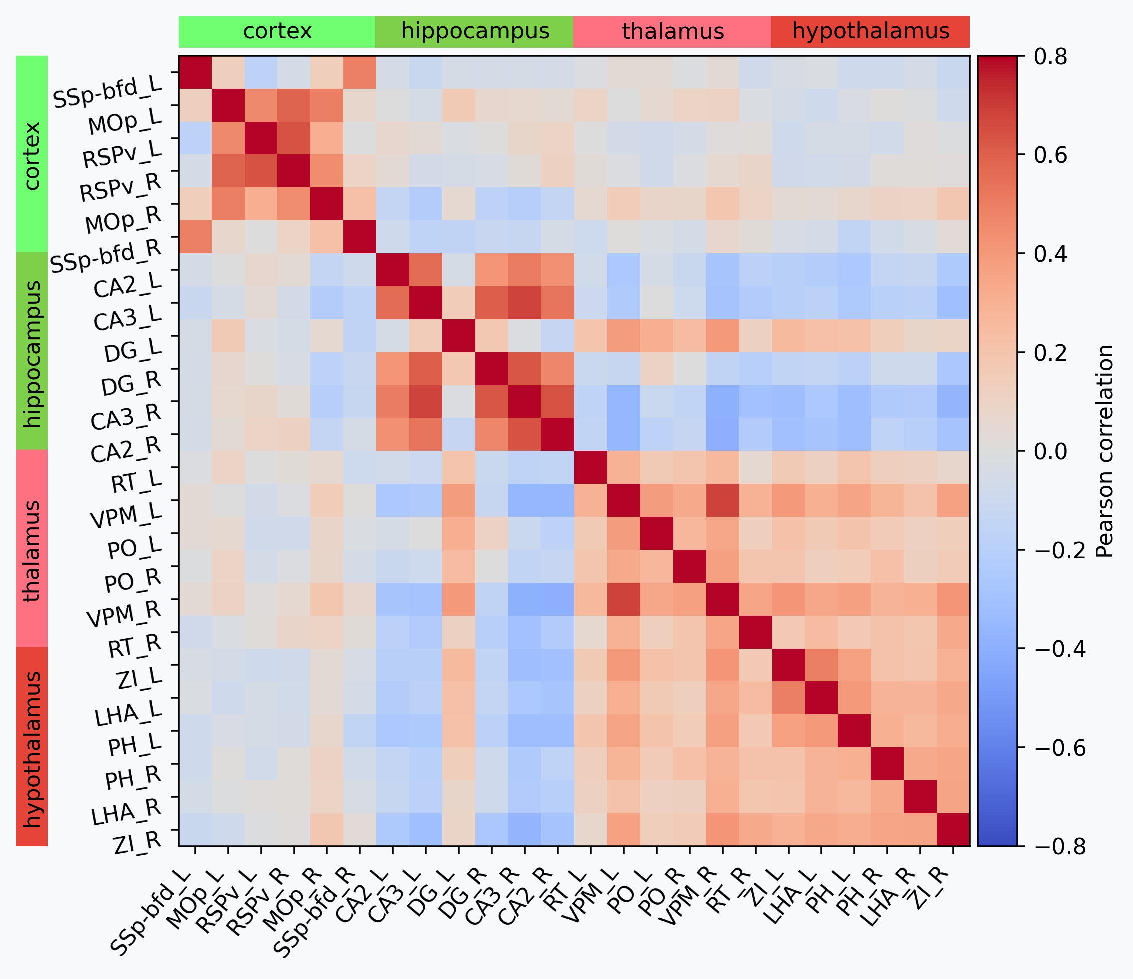
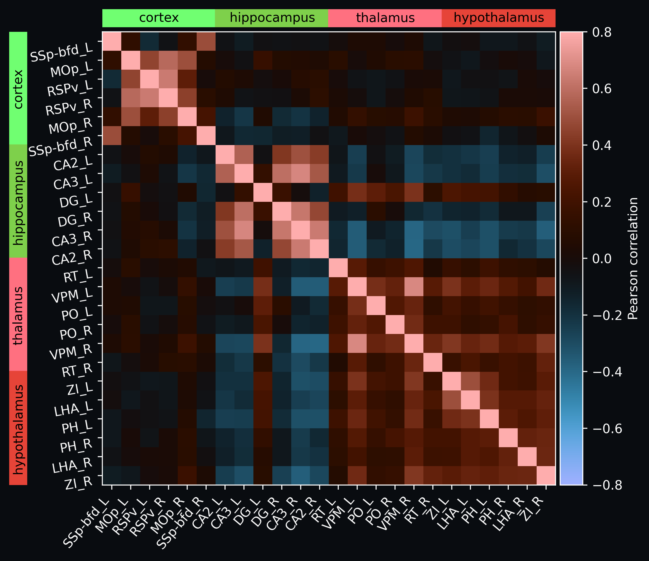
Compute and plot the correlation matrix
ConnectivityMatrix computes the Pearson
correlation matrix between all region pairs from the (time, region) signals.
plot_matrix's groups parameter annotates
contiguous blocks of regions with colored strips—handy here to keep track of which
brain area each region belongs to without cluttering the plot with per-region colors.
group_colors lets us reuse the atlas's own official colors for each area, computed
above from atlas.lookup, instead of arbitrary ones.
fig, ax = cf.plotting.plot_matrix(
    connectivity,
    labels=region_order,
    groups=group_labels,
    group_colors=group_colors,
    vmax=0.8,
    cbar_label="correlation",
    title="Region correlation matrix",
    bg_color=bg_color,
)
Total running time: 187.3 s