Atlas-based seed connectivity maps¶

This example computes voxel-wise seed-based functional connectivity maps: register a single-slice fUSI recording to an Allen-space template, bring an Allen Mouse Brain Atlas into the recording's native space, pick four atlas regions of interest as seeds, and correlate each seed's signal against every voxel with SeedBasedMaps. Each resulting map is displayed with plot_stat_map, using the resampled Allen reference volume as background.

We use an awake freely-running acquisition from subject CR022, session 20201007, in the Nunez-Elizalde 2022 dataset¹, and the Pepe, Mariani 2026 fUSI template, which carries the affine transform required to bring it into Allen Common Coordinate Framework (CCF) space. For the full registration workflow, see Register a recording to an Allen fUSI template.

Fetch the recording and register to the Allen atlas¶

The recording is a single coronal slice imaged for approximately 4 minutes at 3.33 Hz. Registration works on a static anatomical image, so we use the temporal mean, converted to decibels for a more stable dynamic range.

from pathlib import Path

import matplotlib as mpl
import matplotlib.pyplot as plt
import numpy as np
import xarray as xr

import confusius as cf

# Adapt background color to the current Matplotlib style.
bg_color = mpl.colors.to_hex(mpl.rcParams["figure.facecolor"])

xr.set_options(display_expand_data=False)

template = cf.datasets.fetch_template_pepe_mariani_2026().compute()

bids_root = cf.datasets.fetch_nunez_elizalde_2022(
    subjects="CR022", sessions="20201007", tasks="spontaneous", acqs="slice02"
)

If you use this template in your work, please cite the following source:

Pepe, C., Mariani, J.-C., Urosevic, M., Gini, S., Stuefer, A., Ricci, F., Galbusera, A., Iurilli, G., & Gozzi, A. 
(2026). Structural and dynamic embedding of the mouse functional connectome revealed by functional ultrasound 
imaging (fUSI). bioRxiv. https://doi.org/10.64898/2026.02.05.704055

If you use this dataset in your work, please cite the following source:

Nunez-Elizalde, A. O., Krumin, M., Reddy, C. B., Montaldo, G., Urban, A., Harris, K. D., & Carandini, M. (2022). 
Neural correlates of blood flow measured by ultrasound. Neuron, 110(10), 1631–1640.e4. 
https://doi.org/10.1016/j.neuron.2022.02.012

data_path = (
    Path(bids_root)
    / "sub-CR022"
    / "ses-20201007"
    / "fusi"
    / "sub-CR022_ses-20201007_task-spontaneous_acq-slice02_pwd.nii.gz"
)
# The recording's timepoints are not perfectly uniformly spaced so we resample to a
# uniform grid before any time-domain processing (filtering below requires it).
data = cf.timing.resample_to_uniform_time(cf.load(data_path))
moving = data.mean(dim="time").fusi.scale.db().compute()

/tmp/ipykernel_52731/3634357438.py:10: UserWarning: Time coordinate is non-uniform; using the median step to build a uniform target grid.
  data = cf.timing.resample_to_uniform_time(cf.load(data_path))

We don't describe the registration process here to keep the notebook focused on seed-based connectivity, but the key steps are:

• Get an initial affine transform using napari's "Transform" tool.
• Use register_volume to refine the alignment.
• Resample the Allen atlas into the recording's native space with resample_like.

For the full walkthrough, see Register a recording to an Allen fUSI template.

napari_affine = np.array(
    [
        [1.0, 0.0, 0.0, 5.594638656430411],
        [0.0, 1.0, 0.0, -2.50293925701927],
        [0.0, 0.0, 1.0, 5.6650243788545875],
        [0.0, 0.0, 0.0, 1.0],
    ]
)
initialization = np.linalg.inv(napari_affine)

# Crop the template to a thin band around the recording's expected location to improve
# registration speed and visualization.
target_z = napari_affine[0, 3] + moving.fusi.origin["z"]
fixed = template.sel(z=slice(target_z - 1.0, target_z + 1.0))

registered, affine, diagnostics = cf.registration.register_volume(
    moving=moving,
    fixed=fixed,
    transform_type="affine",
    metric="correlation",
    convergence_window_size=100,
    number_of_iterations=500,
    learning_rate=1,
    initialization=initialization,
    show_progress=False,
)

world_to_sform = template.attrs["affines"]["world_to_sform"]
subject_to_atlas = world_to_sform @ np.linalg.inv(affine)

atlas = cf.datasets.fetch_brainglobe_atlas("allen_mouse_100um", check_latest=False)
atlas_native = atlas.atlas.resample_like(moving, subject_to_atlas)

/home/runner/work/confusius/confusius/src/confusius/datasets/_brainglobe.py:235: UserWarning: BrainGlobe provides no mesh for region id(s) ['545'] of atlas 'allen_mouse_100um'; requesting their mesh will fail.
  _fetch_all_meshes(atlas)

Choose seed regions¶

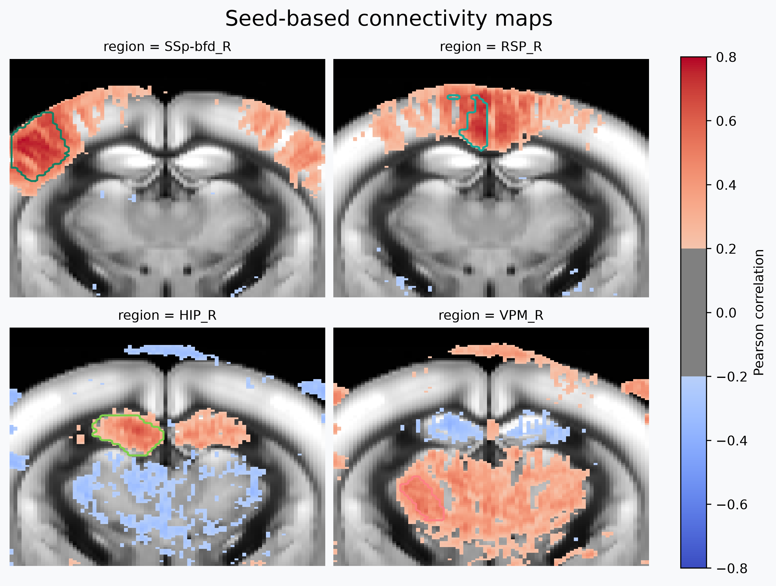
We pick one seed from each of four functional systems, to contrast their connectivity patterns: the primary somatosensory barrel field cortex ("SSp-bfd"), a classic resting-state seed with a strong, well-documented bilateral (interhemispheric) correlation signature; the retrosplenial cortex ("RSP"), a default-mode-like hub expected to correlate broadly across much of cortex; the hippocampus ("HIP"), which should instead correlate with a more localized, hippocampal-formation-restricted network; and the ventral posteromedial thalamic nucleus ("VPM"), a somatosensory relay nucleus expected to correlate with "SSp-bfd" through the thalamocortical pathway. All seeds are taken from the right hemisphere only, so that any left-hemisphere correlation in the resulting maps reflects genuine interhemispheric connectivity rather than the seed leaking into its own mask.

get_masks returns a stacked (mask, k, j, i) integer DataArray—one layer per requested region—which SeedBasedMaps accepts directly as seed_masks.

seed_masks = atlas_native.atlas.get_masks(
    ["SSp-bfd", "RSP", "HIP", "VPM"], sides="right"
)

Smooth and compute nuisance regressors¶

We lightly smooth the recording spatially with smooth_volume (0.1 mm FWHM) to improve the voxel-wise SNR before extracting confound signals and fitting the seed-based maps.

As in the correlation-matrix example, we regress out an aCompCor component extracted from white-matter voxels (the Allen ontology's "fiber tracts" division) together with a low_cutoff high-pass cosine filter for slow drift. Both are passed to SeedBasedMaps via clean_kwargs, which cleans the full voxel-wise recording before extracting the seed signals, so seeds and voxels are preprocessed consistently.

data = cf.spatial.smooth_volume(data, fwhm=0.1)

white_matter = atlas_native.atlas.get_masks("fiber tracts").isel(mask=0)
acompcor = cf.signal.compute_compcor_confounds(
    data, noise_mask=white_matter, n_components=1, variance_threshold=0.95
)

Compute the seed-based correlation maps¶

SeedBasedMaps extracts each seed's average signal, correlates it against every voxel in the recording, and returns one Pearson r map per seed, stacked along a region dimension.

mapper = cf.connectivity.SeedBasedMaps(
    seed_masks=seed_masks,
    clean_kwargs={"low_cutoff": 0.01, "filter_method": "cosine", "confounds": acompcor},
)
mapper.fit(data)
mapper.maps_

Plot the seed maps¶

Each seed's map is plotted with plot_stat_map over the resampled Allen reference volume, with vmax=0.8 fixing the colormap to a shared range so the four seeds are directly comparable. mapper.maps_ stacks all four seed maps along a region dimension, so a single plot_stat_map call with slice_mode="region" plots one panel per seed as long as the background is broadcast to the same region dimension first. We outline each seed's own ROI with VolumePlotter.add_contours, leaving colors unset so each region is drawn in its canonical Allen color (read from the atlas mask's attrs["cmap"]/attrs["norm"], the same convention used by get_masks elsewhere).

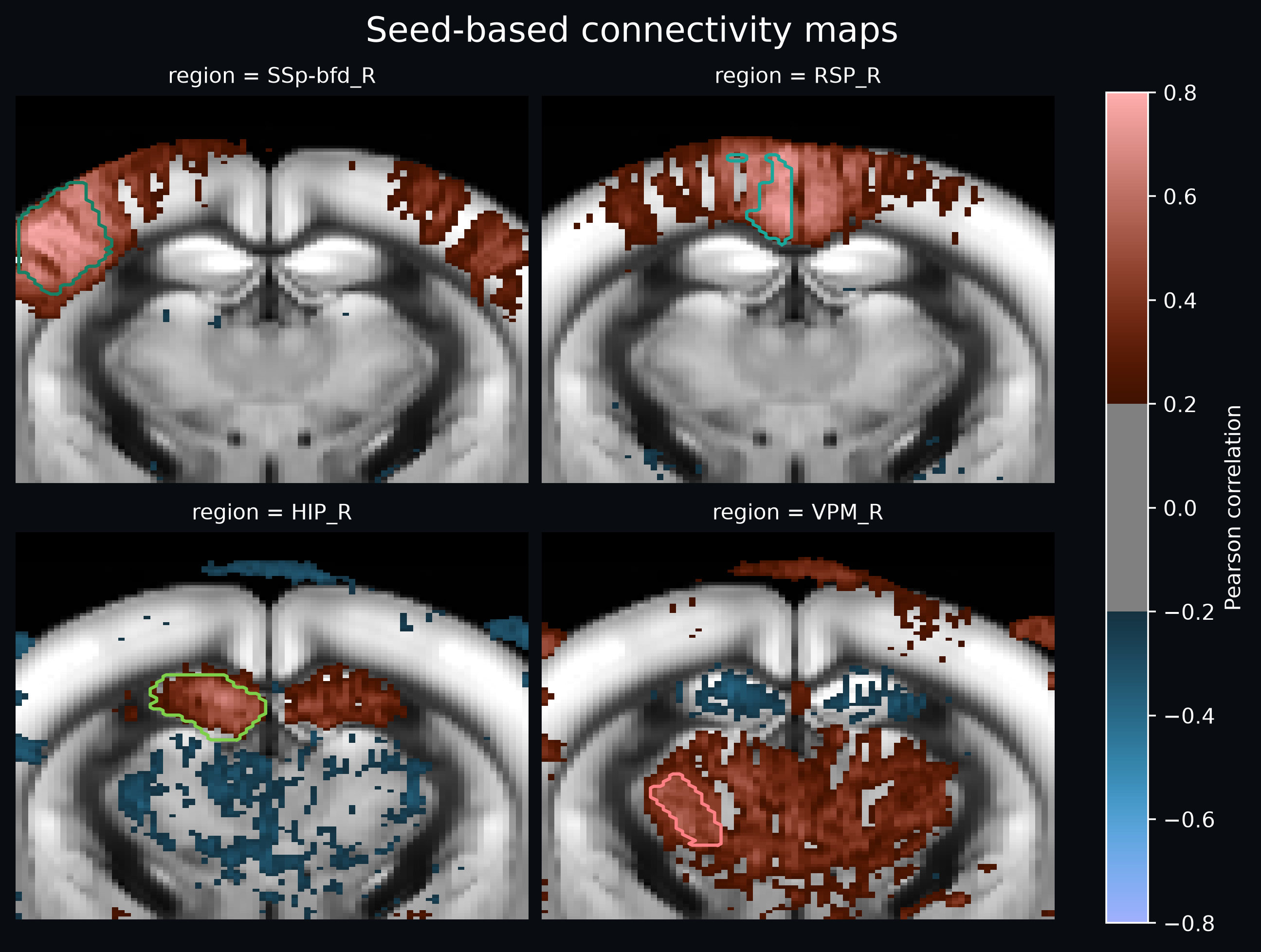
# coolwarm's white midpoint reads as a washed-out hole on a dark background, so switch
# to berlin (Crameri's perceptually uniform diverging colormap, black midpoint) when the
# current Matplotlib style is dark.
is_dark_theme = sum(mpl.colors.to_rgb(bg_color)) / 3 < 0.5
cmap = "berlin" if is_dark_theme else None

# Broadcast the shared background and brain outline across a "region" dimension
# matching mapper.maps_, so plot_stat_map can slice both by region in one call.
bg_by_region = atlas_native.reference.expand_dims(region=mapper.maps_.region)

fig, axes = plt.subplots(2, 2, figsize=(8, 6), constrained_layout=True)
fig.patch.set_facecolor(bg_color)

plotter = cf.plotting.plot_stat_map(
    mapper.maps_,
    bg_volume=bg_by_region,
    slice_mode="region",
    cmap=cmap,
    vmax=0.8,
    threshold=0.2,
    cbar_label="Pearson correlation",
    show_axes=False,
    figure=fig,
    axes=axes,
    bg_color=bg_color,
)
plotter.add_contours(seed_masks.rename(mask="region"), linewidths=1.5)

_ = fig.suptitle("Seed-based connectivity maps", fontsize=16)

Total running time: 17.4 s

Launch in Binder Download .py Download .ipynb